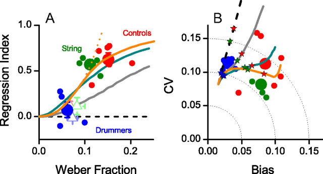
Figure 3.

A, Regression index plotted against Weber fraction for interval bisection. The regression index is the deviation from veridicality of the linear fit to reproduction data like those of Figure 2 (0 for veridicality, 1 for total regression to the mean). Small symbols are individual subjects; large symbols are groups (blue, drummers; green, string musicians; red, controls). Filled circles show results for the visual task, open triangle for audition. The curves show the no-prior model (dashed black), Jazayeri and Shadlen's (2010) BLS model (gray), our Bayesian model (Fig. 1B) with prior of fixed width of 120 ms (cyan), and the Bayesian model where the width of the prior is chosen to optimize performance following the procedure of Figure 4 (orange). The continuous curve shows the model where the width of the prior is curtailed to remain >90 ms (estimated to best fit the data), the dashed where it is free to become infinitely narrow. B, CV (normalized average root variance of the reproductions) plotted against bias (difference between average production time and physical sample interval) for visual reproductions for the three subject groups (colors as in A). The total error (root mean squared error) is given by the distance from the origin, similar for the three groups. The continuous curves show simulations of the models in A, assuming the existence of a further nonsensory noise source, assumed to be constant for all subjects, and optimized to provide best overall fit of data (in practice a Weber fraction of 0.1). Each curve was created by varying sensory Weber fraction from 0.01 to 0.3: the colored stars superimposed indicate the average Weber fractions for that subject group.