Figure 3.

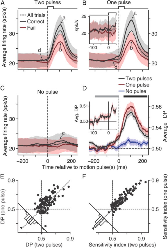
Population analysis of neural–behavior covariations. The average population firing rate over time for correct (black), failed (red), and all (dashed) trials for two motion pulses occurring simultaneously in both RFs (A), one motion pulse in the RF (B), or no motion pulse in the RF (C). Data were computed with a 100 ms sliding window. The inset in B shows the population average firing rate computed with a 10 ms sliding window combining both the one- and two-pulse conditions. Arrows indicate comparison time points for one- and two-pulse correct (a) and failed (b) neural responses, no pulse trials (c), and early divergence between correct and failed responses (d). D, The population average DP over time for two motion pulses occurring simultaneously in both RFs (black), one motion pulse in the RF (red), or no motion pulse in the RF (blue), computed with a 100 ms sliding window. The inset shows DP computed with a 10 ms sliding window combining both the one- and two-pulse conditions. E, DP computed from trials with one motion pulse in the RF versus DP computed from trials with two motion pulses in both RFs. DP was computed using the 200 ms window (black bar) in D. F, Sensitivity index (which measures signaling reliability, see Materials and Methods) computed from trials with one motion pulse versus the sensitivity index computed from trials with two motion pulses. Sensitivity index was computed using the two 200 ms windows (gray and black bars) in D. For both E and F, each data point represents one neuron, marginal histograms show the paired difference between the one- and two-pulse conditions, and triangles show the median difference. Shaded areas denote SEM.