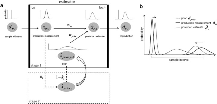
Figure 2.
Two-stage Bayesian estimator model on logarithmic scales. a, Schematic estimation process. Stage 1, The produced displacement dp,i in trial i is represented by the Bayesian estimator as a measurement likelihood on logarithmic scales p(xm,i). The posterior estimate of displacement is determined by the weighted average of the measurement xm,i and an a priori estimate of displacement x̂prior,i−1, with weights of measurement wm and prior wprior, resulting after backtransform in a reproduced displacement on linear scales dr,i. Stage 2, The posterior estimate of the prior in trial i, x̂prior,i, is estimated before the next trial according to the weighted average of the a priori estimate x̂prior,i−1 and the measurement xm,i, with weights ki and 1 − ki, modeled by the discrete formulation of the Kalman filter, where ki refers to the Kalman gain. The posterior is updated over time to build the prior estimate x̂prior,i−1 in the subsequent trial. b, Example for the effect of the Bayesian estimator model on linear scales for a particular sample interval. If the prior dprior is close to the mean of the sample interval, Bayesian fusion with the measurement dm leads to a posterior estimate dr that overestimates small displacements and underestimates large displacements. The effect is stronger for larger displacements (black arrows), due to the calculation of the weighted average on logarithmic scales and thus an increased standard deviation with increasing mean on linear scales.

