. 2019 Jun 13;8:e45545. doi: 10.7554/eLife.45545

Figure 3. Loss of astrocytic Shh signaling impairs structural plasticity.

(A–C) Example dendrite segment imaged repeatedly over 6 weeks. Day 0 indicates the first day of imaging, subsequent imaging days indicated. White arrows, stable spines; cyan arrows, transient spines; orange arrows, filopodia. (D) Turnover ratios in WT (n = 3–5 animals per age group) and Gfap Smo CKO juvenile mice (n = 4 animals per age group) analyzed over 2 days. (E) Turnover ratios in WT (n = 8 animals) and Gfap Smo CKO (n = 8 animals) adult mice analyzed over 7 days. Statistical analysis by two-way ANOVA, Tukey’s post hoc test (D) and unpaired Student’s t-test (E). (F) Fraction of protrusions identified as filopodia in juvenile (WT, n = 7 animals; Gfap Smo CKO, n = 10 animals) and adult mice (WT, n = 16: Gfap Smo CKO, n = 7 animals). Statistics by two-way ANOVA, Tukey’s post hoc test. (G) Comparison of spine survival curves for WT and Gfap Smo CKO neurons. Each dashed curve represents the curve from an individual mouse (WT, n = 7 animals; Gfap Smo CKO, n = 5 animals). Solid curves represent best-fits to exponential decay models. (H) The fraction of spines belonging to the stable, recurrent, and transient populations. Statistical significance was assessed by Student’s t-test for each class (stable, recurrent, or transient; n = 7 and 8 animals, WT and Gfap Smo CKO, respectively). Stable, p=0.0485; Recurrent, p=0.1023; Transient, p=0.7709. (I) Breakdown of spine morphology in juvenile mice. Statistical analysis by unpaired Student’s t-test for each spine class. For graphs D-F and I, data points represent individual animals, bars represent mean ± SEM.

Figure 3—source data 1. Spine turnover data.
DOI: 10.7554/eLife.45545.014
Figure 3—source code 1. MATLAB-based custom-written code for longitudinal analysis of spine dynamics.
SpineTracking generates a longitudinal tracking file that stores the x,y,z location of each feature, along with its status (missing/present/filopodia) for each tile, LongSurvival gathers all the tiles and pools the data to give the final survival curves for each mouse, and FeatLong is used for examining each feature individually.
DOI: 10.7554/eLife.45545.015

Figure 3.

Figure 3—figure supplement 1. Classification of protrusions.

Figure 3—figure supplement 1.

(A–C) Several examples of protrusions classified as mushroom (blue arrowheads) or intermediate (yellow arrowheads) spines, and filopodia (pink arrow- heads). Note the thin stalk and small bulbous head of the intermediate spine in A, whereas filopodia lack a discerible head (B and C). (D) The fraction of protrusions classified as mush- room or intermediate in adult Gfap Smo mice and WT controls. Data points represent individual animals, bars represent mean ± SEM. Statistical analysis by unpaired Student’s t-test.
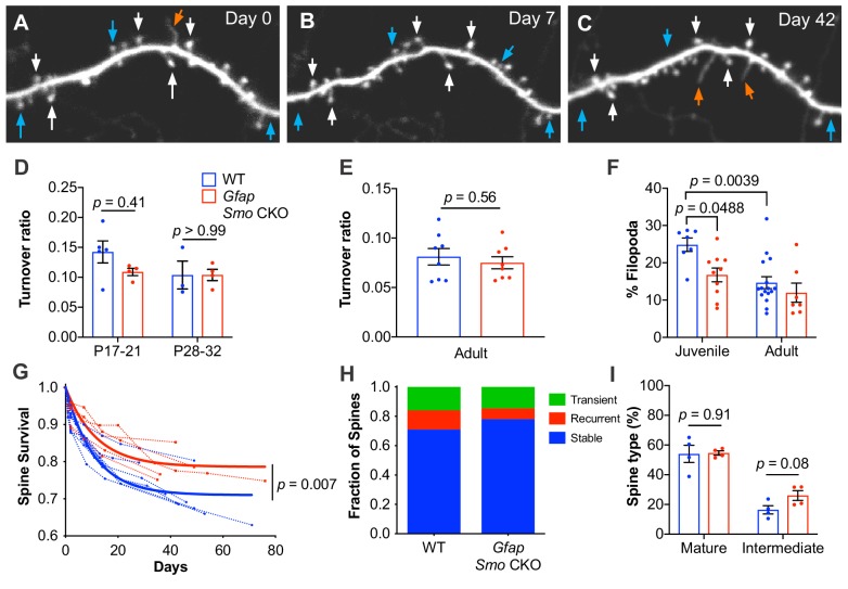
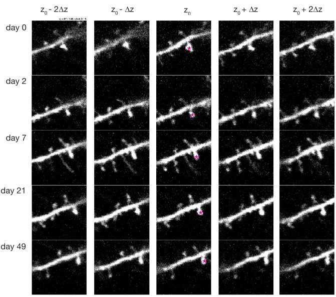
Figure 3—figure supplement 2. Screenshot depicting the graphical user interface used for longitudinal tracking of spines across multiple days of imaging.

Figure 3—figure supplement 2.

A spine identified in the first imaging session (pink star, top central panel) is presented to the user for scoring. The same spine is manually tracked across subsequent days (rows). For each day, multiple frames above and below the estimated z-plane corresponding to that spine, Z0, are also presented (columns). For each timepoint, the user then clicks on the spine’s head using the frame that best captures the spine. In this case, the frame jump, Δz, was set to 1, and four neighboring frames are presented; these parameters can be adjusted as necessary.