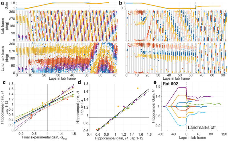
Figure 3 |. Recalibration of place fields by landmarks.

a, Example of positive recalibration. (top) Experimental gain, G (blue) and hippocampal gain, H (yellow) for Epochs 1–3 of a session in which the G_final was 1.769. (middle) Spikes from three putative pyramidal cells (blue, red and yellow dots) in the lab frame. (bottom) The same spikes in the landmark frame. When the landmarks were turned off (dashed line, Epoch 4), H remained close to G_final, shown by the slower drift of the place fields in the landmark frame compared to the lab frame. (During Epoch 4, the landmark frame was defined assuming the gain was G_final even though landmarks were off.). Note that the traces of H (yellow) deviate from G (blue) prior to the landmarks turning off; this is an artifact of the sliding window used in the spectrogram and does not affect the conclusions (see Methods, Visualizing H). b, Example of negative recalibration. The G_final was 0.539. c, Recalibration of place fields. The x-axis is G_final and the y-axis is H computed using the first 12 laps (i.e., the value of H at lap 6) after the landmarks were turned off. Linear fits for each animal (color) and for the whole data set (black) are shown (n = 45 sessions, Pearson’s r₄₃ = 0.94, p = 3.4 × 10⁻²¹), along with the perfect recalibration line (dashed line, black). Note that the linear fit passes close to the origin, showing that H≈1 when the landmarks were extinguished after baseline control experiments. d, Stability of recalibration. Comparison of H during laps 1–12 vs. H during laps 13–24. The linear fit is shown in black. (n = 27 sessions, Pearson’s r₂₅ = 0.96, p = 1.16 × 10⁻¹⁵) e, Complete gain dynamics for one animal. For all sessions from one rat, H is plotted as a function of laps run in the lab frame. All the sessions are aligned to the instant when the landmarks were turned off (lap 0). The recalibrated H was maintained for as many as 50 laps or more.