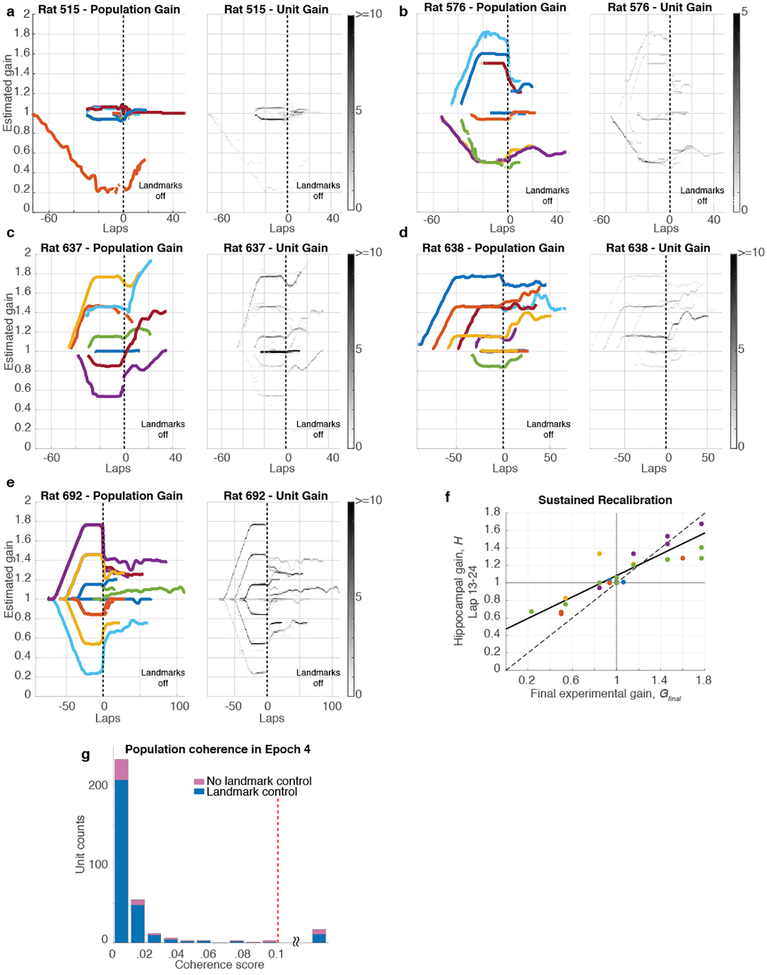
Extended Data Figure 6: Dynamics of recalibration.

a-e. The complete hippocampal gain (H) dynamics for all 5 rats for trials that exhibited landmark control. (The gain dynamics for Rat 692 is also shown in the main text, Fig. 3e.) In the left panels for each rat (color), H is plotted as a function of laps run in the lab frame. Sessions are aligned to the instant when the landmarks were turned off (denoted as lap 0). In the presence of landmarks, (before lap 0), the hippocampal gain tracked the experimental gain profiles during a given session (not shown). After the landmarks turned off, the traces largely maintained their recalibrated gain, while also showing some variable drift across experiments. Note that for each rat, for experiments in which G = 1 (i.e., the landmarks did not move), the value of H was close to 1 when the landmarks were extinguished. The right panels for each rat show the gain trajectories of all the units in the dataset. The gray scale represents the number of active cells with gains falling in a given bin (bin size is 5° for laps axis and 0.01 for gain axis). These graphs demonstrate the high degree of coherence of the hippocampal population, as almost all cells shared the same gain with minimal deviation. The light-colored lines that occasionally deviate from the main trajectories arise from the small number of cells with poor spatial tuning or from cells that remapped. In the latter case, because our spectral gain analysis used a window of 12 laps, these remapped cells continued to show artefactual values for the limited number of laps that fall in this window but during which the cell was silent. As can be seen, these exceptions had negligible influence on the median population gain values. f, Sustained recalibration. Comparison of G_final (x-axis) and H computed using laps 13–24 (i.e., the value of H at lap 18) after the landmarks were turned off (y-axis). Sessions for each rat are plotted in different colors, along with the perfect recalibration line (dashed line, black) and a linear fit (solid line, black; n = 27 sessions, Pearson’s r₂₅ = 0.85, p = 2.04 × 10⁻⁸). The number of data points is lower than in Fig. 3c because some experiments ended prior to lap 24. g. Histogram of coherence scores (same format as Fig. 2g) for units firing during Epoch 4 (landmarks off). The shape of the histogram is very similar to Fig. 2g. Almost all units had a coherence score below 0.1, indicating that the place fields acted as a coherent population in sessions with (blue) and without (pink) landmark control in Epochs 1–3, even after landmarks were turned off. Units with coherence score above 0.1 (range 0.11 – 0.41) were combined in a single bin (17/336 units).