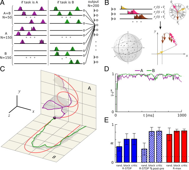
Figure 4.

Results applied to a more realistic spatiotemporal trajectory-learning task. The learning set-up was different from that of Figure 1 in several ways. A, Stochastic input. The firing rates of the inputs are sums of a fixed number of randomly distributed Gaussians. Firing rates (colored areas) are constant over trials, but the spike trains vary from trial to trial (black spikes). Tasks A and B are randomly interleaved. A fraction of inputs fires both on presentation of tasks A and B, the other neurons fire only for a particular task. The network structure is the same as in Figure 1, but with 350 inputs and 200 neurons. B, Population vector coding. The spike trains of the output neurons are filtered to yield postsynaptic rates r_i(t) (upper left). Each output neuron has a preferred direction, υ⃗_i (upper right); the actual direction of motion is the population vector, $\overrightarrow{\upsilon }\left(t\right)={\displaystyle {\sum }_i{r}_i\left(t\right)}{\overrightarrow{\upsilon }}_i/\parallel {\displaystyle {\sum }_i{r}_i\left(t\right)}{\overrightarrow{\upsilon }}_i\parallel$ (bottom right). The preferred directions of the neurons are randomly distributed on the three-dimensional unit sphere (bottom left). C, Reward-modulated STDP can learn spatiotemporal trajectories. The network has to learn two target trajectories (red traces) in response to two different inputs. Target trajectory A is in the xy plane and B is in the xz plane. The green and blue traces show the output trajectory of the last trials for tasks A and B, respectively. Gray shadows show the deviation of the trajectories with respect to their respective target planes. The network learned for 10,000 trials, using the R-max learning rule with critic. D, The reward is calculated from the difference between learned and target trajectories. The plot shows the scalar product of the actual direction of motion υ⃗ and the target direction υ⃗*, averaged over the last 20 trials of the simulation; higher values represent better learning. The reward given at the end of a trial is the positive part of this scalar product, averaged over the whole trial, $R_n=\frac{1}{T}{{\displaystyle {\int }_0^T\left[\overrightarrow{\upsilon }\left(t\right)\cdot \overrightarrow{\upsilon }*\left(t\right)\right]}}_{+}\text{d}t$. E, Results from the spike train learning experiment apply to trajectory learning. The bars represent the average reward over the last 100 trials (of 10,000 trials for the whole learning sequence). Error bars show SD for 20 different trajectory pairs. Each learning rule was simulated in three settings, as follows: randomly alternating tasks with reward prediction system (critic), tasks alternating in blocks of 500 trials without critic (block), and randomly alternating tasks without critic (rand.). The hatched bars represent R-STDP without a post-before-pre window, corresponding to λ = 0 in Figure 2E. The dotted line shows the performance before learning.