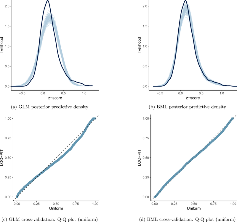
Figure 3:

Model performance comparisons through posterior predictive checks and cross validations between conventional univariate GLM (a and c) and BML (b and d). The subfigures a and b show the posterior predictive density overlaid with the raw data from the 124 subjects at the 21 ROIs for GLM and BML, respectively: solid black curve is the raw data at the 21 ROIs with linear interpolation while the fat curve in light blue is composed of 100 sub-curves each of which corresponds to one draw from the posterior distribution based on the respective model. The differences between the two curves indicate how well the respective model fits the raw data. BML fitted the data better than GLM at the peak and both tails as well as the skewness because pooling the data from both ends toward the center through shrinkage clearly validates our adoption of BML. The subfigures c and d contrast GLM and BML through cross-validation with leave-one-out log predictive densities through the calibration of marginal predictions from 100 draws; the calibration is assessed by comparing probability integral transformation (PIT) checks to the standard uniform distribution. The diagonal dished line indicates a perfect calibration: there are some suboptimal calibration for both models, but BML is clearly a substantial improvement over GLM. To simulate the posterior predictive data for the conventional ROI-based approach (a and c), the Bayesianized version of GLM (15) was adopted with a noninformative uniform prior for the population parameters.