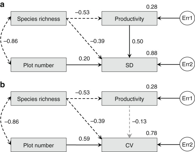
Fig. 7.

Structural equation model showing the connections between biodiversity, productivity, and variability. The grouping of plots is consistent with Fig. 6 (N = 47 plot groups). Variability was measured either as the standard deviation (a), or as the coefficient of variation (b) of productivity across plots within each level of species richness. Solid and dashed one-way straight black arrows represent positive and negative effects, respectively. The one-way gray arrow represents an insignificant (P > 0.05) effect. Dashed two-way black arrows represent negative correlations. To avoid zero degree of freedom, the ‘productivity’ variable in b was not dropped from the model. The exogenous unobserved variables err1 and err2 accounted for the unexplained errors in the estimation of productivity and productivity variability, respectively. Productivity data was ln-transformed before analyses to ensure normality. Test statistic = 0.863, with one model degree of freedom and P = 0.353 for both, indicating close model-data fit. Standardized regression weights (along one-way arrows), correlations (along two-way arrows) and squared multiple correlations (beside Productivity, SD, and CV boxes) for the best-fitting model are shown. Source data are provided as a Source Data file