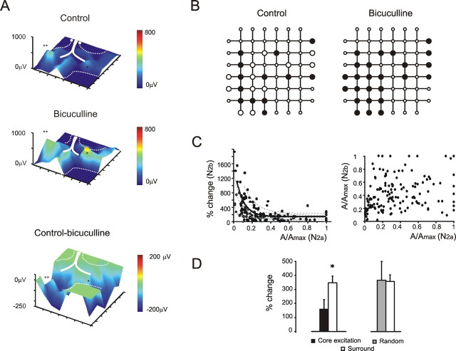
Figure 5.

The relationship between excitation and inhibition. A, Electrical 3D maps show N_2b amplitude before and after application of 10 μm bicuculline. Bicuculline disinhibited several areas. The distribution and intensity of the inhibitory effect is demonstrated by the subtraction map (control − bicuculline). B, In the same slice shown in A, the number of electrodes measuring a detectable N_2b response after bicuculline application (black dots) is increased. Note that N_2a was already measurable over the electrodes showing N_2b after bicuculline application (large open dots). C, Left, Plot of N_2b changes caused by bicuculline as a function of N_2a amplitude. The plot reveals a strong negative correlation between the parameters. The thick line is a monoexponential fitting to the whole dataset [y = y₀ + A × exp(−x/τ), with y₀ = 95, x₀ = 0, A = 1174, τ = 0.09; p(χ²) < 0.001; R² = 0.72; n = 180 in 7 slices], the thin dashed lines are fittings to single-slice data (always R² > 0.6). Right, Plot of N_2b versus N_2a initial amplitude from the same slices: note the absence of correlation. For each slice, N_2a and N_2b amplitudes are normalized to their maximum control value. D, The histogram shows the average change caused by bicuculline in the electrodes with a local peak of excitation versus the surrounding ones. The effect of bicuculline is stronger in the surround (n = 60 from 7 slices; *p < 0.03, paired t test). No comparable difference is observed by random sampling the granular layer electrodes and measuring the surrounding activity (n = 60 from 7 slices; p = 0.74, paired t test). Error bars indicate SEM.