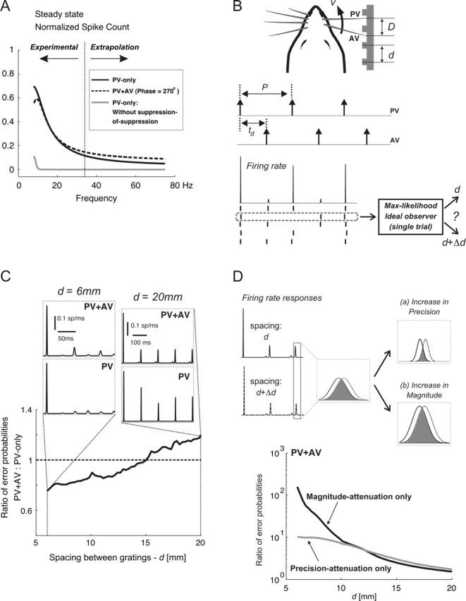
Figure 7.

Limits to discrimination performance for single- and two-vibrissa stimuli. A, Simulated normalized PV spike counts in response to PV-only (solid line) and paired-vibrissa (dashed line; PV–AV phase, 270°) stimuli; all simulations were based on the response model described in Results. The CTR curves used in simulations were obtained by parametrically fitting sigmoidal functions to population-averaged CTR curves. The gray curve shows the simulated PV-only response in the absence of suppression-of-suppression. The range of frequencies for which the response model was verified experimentally, along with the range over which the model was extrapolated are labeled as Experimental and Extrapolation, respectively. B, The whisking model generates idealized single- and paired-vibrissa pulse deflections characterized by their occurrence times. With simple geometrical considerations, the stimulation period P and the PV–AV time delay td are expressed as follows: P = d/v and td = (D mod d)/v, where d, v, and D represent the grating spacing, vibrissa-tip velocity, and inter-vibrissa separation, respectively. For a given geometry and the resulting deflection times, the model described in Materials and Methods generates a pair of firing-rate responses corresponding to surface gratings of d and d + Δd; an example of the firing rate and response rasters is shown. Next, an ideal observer matches the spiking response to the texture that most likely gave rise to that response. C, This plot shows, as a function of grating spacing, the ratio of Perror with two vibrissae to that obtained using only the PV. In all cases, Δd = 0.05 mm. Qualitatively similar results were obtained for other Δd values, although absolute performance improved with increasing Δd (data not shown). D, Changes in Perror as a result of spatiotemporal interactions are attributed to changes in response precision (a) and response magnitude (b). The firing rate responses evoked by spacings of d and d + Δd are shown on the left; the responses to a single stimulus cycle are considered in more detail. For a pair of equally likely surfaces, Perror based on single-trial observations (spikes) of a single response cycle scales with the extent of temporal overlap between the two firing rates; this overlap is shown by the shaded area. An increase in response precision reduces the temporal overlap between the pair of responses (a). In contrast, an increase in response magnitude (b) does not change the fractional overlap between the two responses. It lowers Perror by increasing the likelihood of observing one or more spikes in response: without spikes, Perror is at its maximum (i.e., one-half).
