Machine-learning based classification of glioblastoma using delta-radiomic features derived from dynamic susceptibility contrast enhanced magnetic resonance images

Abstract

Background

Glioblastoma is the most aggressive brain tumor with poor prognosis. The purpose of this study is to improve the tissue characterization of these highly heterogeneous tumors using delta-radiomic features of images from dynamic susceptibility contrast enhanced (DSC) magnetic resonance imaging (MRI).

Methods

Twenty-five patients with histopathologically confirmed to be 13 high-grade (HG) and 12 low-grade (LG) gliomas who underwent the standard brain tumor MRI protocol, including DSC MRI, were included. Tumor regions on all DSC MRI images were registered to and contoured in T2-weighted fluid-attenuated inversion recovery (FLAIR) images. These contours and its contralateral regions of the normal tissue were used to extract delta-radiomic features before applying feature selection. The most informative and non-redundant features were selected to train a random forest to differentiate HG and LG gliomas. Then a leave-one-out cross-validation random forest was applied to classify these tumors for grading. Finally, a majority-voting method was applied to reduce binarization bias and to combine the results of various feature lists.

Results

Analysis of the predictions showed that the reported method consistently predicted the tumor grade of 24 out of 25 patients correctly (0.96). Finally, the mean prediction accuracy was 0.950±0.091 for HG and 0.850±0.255 for LG. The area under the receiver operating characteristic curve (AUC) was 0.94.

Conclusions

This study shows that delta-radiomic features derived from DSC MRI data can be used to characterize and determine the tumor grades. The radiomic features from DSC MRI may be used to elucidate the underlying tumor biology and response to therapy.

Glioblastomas (GBMs) are the most aggressive and lethal brain tumors. Lower grade gliomas [based on the 2007 World Health Organization (WHO) grading scale] have an average relative 2-year survival rate of 80%, while the relative 2-year survival rate for grade IV gliomas drops to only 30% with a median overall survival rate of 12–15 months (1,2). The incidence of malignant gliomas is about 17,000 per year or 5 in 100,000. Overall, about 65% are grade IV which results in a mortality rate of over 10,000 deaths per year (3). These poor outcomes stem from the uncooperative, heterogeneous nature of GBMs where some develop and progress from lower-grade gliomas while others develop as primary tumors (4). Much like other solid tumors, GBMs develop a very heterogeneous pattern of mutations (5). Only recently have there been studies showing the predictive and prognostic power of genetic characterization of GBM (6,7) and expression data correlated with response to treatments (5,8,9). Even so, the genetic and molecular heterogeneity of GBMs still poses a significant hurdle to developing novel therapies and clinical decision making (10). Thus, there is a significant unmet need in accurate characterization and classification of these high-grade (HG) and low-grade (LG) gliomas to select proper treatment options to improve the outcomes of these patients.

In recent years, to circumvent the complexities of intra-tumoral and inter-patient tissue characterization of GBM through sample limited biopsies (11), various imaging modalities have been used to characterize the phenotypic expression of various tumors through the radiomic approach (12-14). With these radiomic approaches, correlations to clinical outcomes have been observed in the breast (15), brain (16), and head and neck (17) by different modalities like computed tomography (CT), positron emission tomography (PET), and magnetic resonance imaging (MRI).

Brain tumor patients typically undergo extensive MRI scans to classify the tumor type, determine the tumor grade, and monitor the treatment response and tumor recurrence (18). Unlike histopathologic analysis of tumor tissue samples collected from biopsies, which cannot reveal intra-tumoral heterogeneity due to sampling limitations, or surgical resection, with its difficulty to repeat, MRI examinations with different imaging techniques can be performed frequently, repetitively, and non-invasively to provide both morphological and physiological information of the tumor with high spatial resolution and tissue characteristics. Among the methods widely used for brain tumors MRI, dynamic susceptibility contrast enhanced (DSC) MRI follows signal intensity changes associated with the passage of intravenously (i.v.) injected paramagnetic contrast agent (e.g., gadopentetate dimeglumine, Gd) through the vascular system to investigate the hemodynamic properties of tissues, such as permeability of the tumor vasculature and blood supplies to the tumor, based on the empirical models of tracer kinetics.

The purpose of this work is to improve the tissue classification of the highly heterogeneous GBMs by taking advantage of: (I) the hemodynamic features that can be derived from DSC MRI data; (II) the delta-radiomic features showing the change in radiomic features over the course of the DSC MRI and/or versus the normal tissue; (III) the random forest machine learning approach which splits observations with similar response variables. This method aims to be able to extract “hidden” delta-radiomic features from DSC MRI data, select and apply the most salient features, and train a random forest to classify HG or LG GBMs with cross validations.

Methods

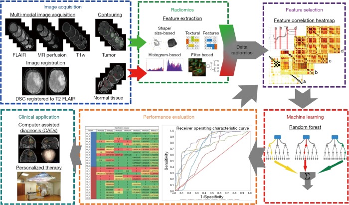
The proposed classification method used in this study is described as in Figure 1. First, MRI images of patients are acquired, registered, and contoured. Then radiomic features are extracted. Afterwards, feature selection is applied to get the most salient features, followed by using random forest decision trees to train and test the classification method. Finally, the performance is evaluated and optimizations are applied.

Figure 1.

The flowchart of our proposed classification method. FLAIR, fluid-attenuated inversion recovery; T1W, T1-weighted.

Image acquisition

Patient data

Image data from clinical brain tumor MRI exams of 25 patients who had biopsy or tumor resection after MRI exams for pathology were selected for retrospective analysis. The use of these MRI data was approved by the Emory institutional review board (IRB) with written informed consent obtained from the study subjects. Among 25 patients, 12 were pathology confirmed HG gliomas, GBMs, and 13 were LG gliomas with tumors located mostly in the frontal or temporal regions of the brain. The tumor grades, classified based on the 2007 WHO grading scale at the time, were determined based on histopathological analysis and none of the cases were recurrent or primary tumors before treatment. Among 25 cases, 17 were assessed with tumor proliferation MIB-1 index based on the Ki-67 assay.

MRI protocol

All patients underwent MRI exams on a 3T MRI scanner (Magnetom Tim/Trio; Siemens, Germany) with a routine brain tumor protocol which included the following MR sequences: pre- and post-contrast enhanced T1-weighted axial, sagittal, and coronal spin-echo imaging, T2-weighted (axial) fluid-attenuated inversion recovery (FLAIR), diffusion-weighted imaging (DWI), and DSC MRI. Axial T2 FLAIR images, which were used for the segmentation of the tumor, were obtained using the following parameters: repetition time/echo time (TR/TE) =6,000/93 ms, flip angle =130°, inversion time =2,030 ms, slice thickness =3 mm, FOV =128×128 mm², and 25 axial slices (thickness =1.875 mm).

DSC MRI data were acquired using a single-shot echo planar sequence with TR =45 ms, TE =2,000 ms, with 50–70 time points, field of view (FOV) of 22 cm, matrix of 128×128. A bolus of 0.05–0.15 mmol/kg gadolinium (Gd) contrast agent was injected at a rate of 3 mL/s at 20 s after starting the dynamic data acquisition.

Image registration and contouring

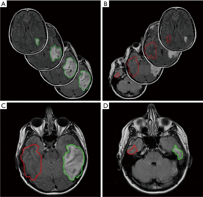
First, the time series DSC images of each patient were performed first using rigid registration by Velocity AI 3.2.1 (Varian Medical Systems, Palo Alto, CA, USA) and then manually adjusted for the small mismatch. They were registered to the corresponding T2 FLAIR image given its superior resolution and tissue contrast. Once all images were registered, the tumor was contoured on the T2 FLAIR images. In order to derive delta-radiomic features, we exported the contours as Matlab matrices and flipped the contours contralaterally to obtain normal tissue contours to contrast against the tumor. Once flipped, these contours were translated to best match the anatomical features of the opposing hemisphere. The contralateral contours from normal tissue were trimmed according to the anatomy, e.g., if any part of the contralateral contour was outside of the brain, crossed the midline, or crossed into the tumor, it was contoured out. After contours of both tumors and normal areas were drawn and shaped to satisfaction, they were applied to the entire volumes of DSC MRI time course data for feature extraction. Figure 2 shows an example of one set of tumor contour, normal tissue contour, and contour trimming from a LG glioma patient.

Figure 2.

Tumor and normal tissue contours. A side by side view of the tumor contour (A) and the contralateral normal tissue contour (B). On the bottom, a side by side view of two image slices (C,D) where the normal tissue contour (red) was trimmed to fit the patient anatomy resulting in a smaller contour than the tumor (green).

Radiomics

Feature extraction

After contouring the images and selecting the features to extract, a total of 1,689 different features were extracted for each image using IBEX (Imaging Biomarker Explorer), an open-source radiomics tool (19). These features were defined as those spatially local and global image features extracted from IBEX. Handcrafted features from IBEX were chosen because they were designed with prior knowledge to balance accuracy and computational efficiency with attention to specific issues in computer vision and image classification like variations in image scale and intensities (20). Deep features from the data itself was considered but not chosen due to concerns of overfitting to the small dataset. Once all features were extracted, following feature transformation methods were applied to calculate delta-radiomic features and normalize the data. While contemporary papers define delta-radiomics as those radiomic features that change over time, usually pre- and post-treatment features, our paper more broadly defines delta-radiomics as those features that change over time or are different to the normal tissue. To extract delta-radiomic features, we used three methods to derive delta-radiomic features: (I) subtraction (absolute difference) to the tumor baseline or feature change over time; (II) absolute difference between tumor features and normal tissue features; and (III) normalization (relative difference) to normal tissue features. These subtraction and normalization derived a matrix of delta-radiomic features, features that change over the DSC image as well as the features that are different than the normal tissue, that were used to create our feature lists (FLs) which were then optimized to our classification method via feature selection. Additional normalization methods were applied to: (I) observe if normalization of features improved our classification method and (II) reduce inter-patient feature variances. Table 1 summarizes a list of the final feature transformations used in the further analyses, corresponding descriptions of these features and how they were derived.

Table 1. Table of final feature lists (FLs).

Feature list name	Feature list description
FL 1	Raw tumor features
FL 2	Delta radiomic features via subtraction of tumor baseline features
FL 3	Delta radiomic features via subtracting normal tissue from tumor features
FL 4	Delta radiomic features via dividing tumor features by normal tissue features
FL 5	FL 3 normalized by subtracting the baseline
FL 6	FL 3 normalized by dividing with the baseline
FL 7	FL 4 normalized by dividing with the baseline

Feature selection

Feature selection was applied once all features were extracted. It is a procedure commonly applied in radiomic and machine learning studies to reduce redundant variables, extract the most informative features and maintain efficiency of computation. The first part of our feature selection was to extract features that showed a significant difference between HG and LG gliomas as well as a preliminary reduction of features. We used a combination of LASSO (least absolute shrinkage and selection operator) and two sample t-test (2Samp) to achieve this. LASSO is a commonly used statistical regression analysis that is used to increase the prediction accuracy of statistical models by selecting unique and significant predictors (21,22). A two-sample t-test is a statistical test used to determine if two population means are equal.

In this case, HG patients and LG patients were considered as two sample populations to select features that are significantly different at the 0.05 significance level and then the first round of LASSO was used to further select and reduce features. After both feature selections were finished, only those features that were selected to be significant by both tests, LASSO and 2Samp (L2S), were chosen to be used in further processes. Once the most significant features have been selected, redundant features were removed using a correlation-matrix-based selection with variable correlation thresholds.

Finally, an additional positive-feature selection was performed after initial performance evaluations. These positive-features were defined as those features that were added with each increasing correlation limit that positively affected the outcome of overall prediction accuracy. This positive-feature selection was applied with the expectation: (I) that it would improve prediction accuracies by removing features that reduced the accuracy of our method; (II) reduce the computational load by significantly reducing the number of features used to train and test the model; (III) extract and observe radiomic and delta-radiomic signatures, combinations of features, and feature groups that are the most informative in classifying tumors for different grades.

Machine learning

Random forest

After feature selection, a random forest machine learning method was used to classify the selected gliomas. Recent studies have used random forests to train the classification or regression model, due to its efficacy in tackling medical image processing (23-26). Random forests train a bag of decision trees, each of which is provided with a random subset of training data and trained independently from the others. This generally yields favorable error rates and are robust to noise (27).

Specifically, we chose to use the Matlab function, fit ensemble, with a semi-optimized template tree without internal cross validation due to the low number of patients and the nature of the patient data, each patient’s DCS volumes being read as “one input”. Since the whole volume, from the start to end volumes of DSC MRI, is treated as “one input”, a class voting method such as random forests, support vector machines, or other methods are useful to obtain a majority vote classification. Although some time point volumes within the DSC MRI may be classified incorrectly, ideally the majority of the volumes will be classified correctly with sufficiently informative features obtained through feature selection. However, support vector machines inherently solve for binary or two-class problems which doesn’t allow future testing of our method in multi-class problems such as classifying tumors by their grades, grades 1–4. Additionally, while other classification methods have a tendency to overfit at low training sizes, random forests are robust against it and are simpler to train and tune (28). At each correlation limit, the corresponding features and labels (of HG or LG patients) for each method were supplied to the random forest to train and test it, resulting in various performance metrics such as prediction accuracy (predicted label), prediction confidence (score), and receiver operating characteristic (ROC) curves.

Performance evaluation

To evaluate the performance of our classification method to the larger population and reduce the overfitting bias, we chose to use a leave-one-out cross validation on the random forest. This allowed our method to be trained and tested over multiple iterations, each with a new test patient. After the leave-one-out cross validation testing, we evaluated the performance of our machine-learning based classification method by calculating the accuracy of our predictions, and calculating the area under the ROC curve (AUC) while stratifying these values by confirmed HG or LG patients. Once each individual FLs were evaluated on its performance, a majority voting method based on the various normalization methods was applied to minimize the strong bias produced from the binarization of a few approaches in the final result. Our results were compared to similar studies and are discussed.

Results

The result for each FL is first provided in. In Table 2. The best result is defined as the correlation threshold at which that FL gave the best average classification accuracy. In Table 3, the results were obtained from positive features derived from the full range of the correlation thresholds to achieve the presented values.

Table 2. Table of best results for each feature list.

Variables	Leave-one-out best
	FL 1 [71]	FL 2 [24]	FL 3 [522]	FL 4 [87]	FL 5 [679]	FL 6 [159]	FL 7 [526]
Average accuracy	0.758	0.784	0.744	0.810	0.821	0.776	0.741
HG accuracy	0.775	0.816	0.698	0.830	0.949	0.861	0.784
LG accuracy	0.740	0.750	0.794	0.789	0.682	0.684	0.694
AUC	0.822	0.314	0.737	0.835	0.797	0.676	0.766

HG, high-grade; LG, low-grade; AUC, area under the curve; FL, feature list.

Table 3. Table of results for each feature list using positive features.

Variables	Leave-one-out positive-features only
	FL 1 [277]	FL 2 [331]	FL 3 [326]	FL 4 [96]	FL 5 [384]	FL 6 [275]	FL 7 [256]
Average accuracy	0.688	0.593	0.718	0.789	0.720	0.760	0.713
HG accuracy	0.747	0.684	0.707	0.793	0.838	0.835	0.771
LG accuracy	0.624	0.494	0.731	0.784	0.592	0.678	0.650
AUC	0.810	0.641	0.763	0.822	0.725	0.811	0.802

HG, high-grade; LG, low-grade; AUC, area under the curve; FL, feature list.

Finally, with the use of our best-majority voting combination method, the best resulting accuracies were 0.902±0.191, 0.950±0.091, and 0.850±0.255 for all, HG, and LG patients, respectively, with an AUC of 0.938.

Results across correlation limits

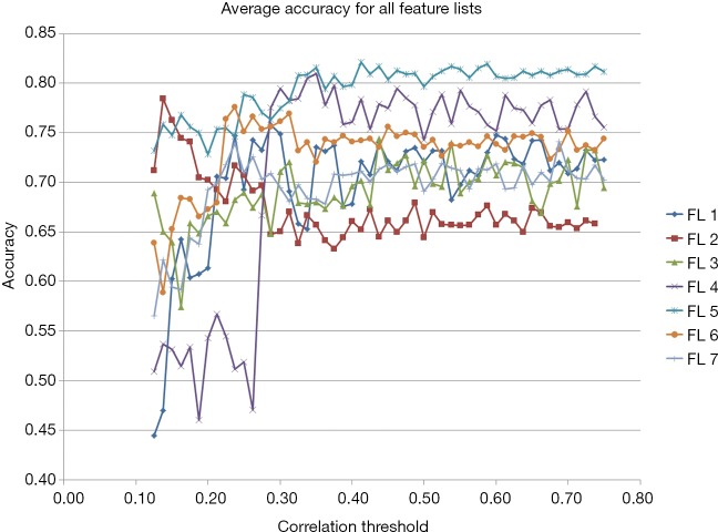
In comparing the various methods of feature manipulation, namely subtraction, absolute difference, and normalized delta-radiomic features, as well as correlation limits, we observed a few trends. For example, the first two feature transformation lists, 1 and 2, show that peak performances occur at lower correlation limits at 28.75% and 13.75%, respectively, while other features showed peak performances at higher correlation limits (Figure 3). Additionally, we found that the delta-radiomic features derived from the differences between the tumor and normal tissue, normalized or not, performed better than those that were not.

Figure 3.

Performance of selected features. Graphs of accuracy across correlation thresholds of different feature lists. As shown in the graph, FL 5 has the best average accuracy at 0.821. FL, feature list.

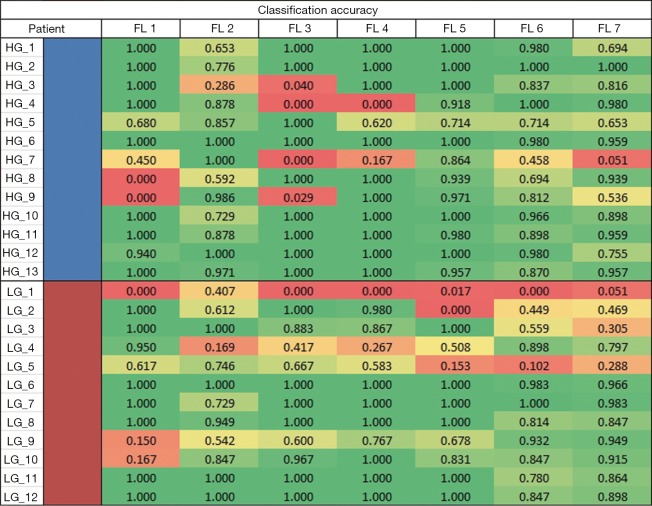
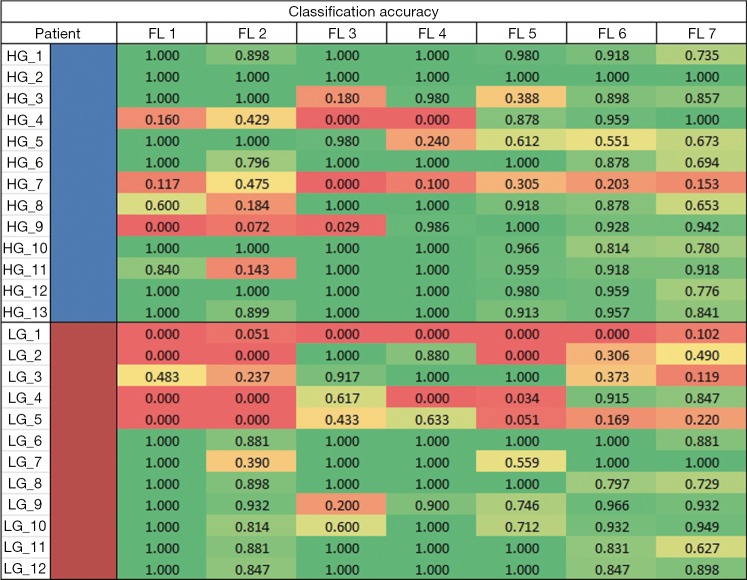
Looking at the peak accuracies for all transformed FLs, we derived an accuracy heatmap by stratifying the accuracies by patients and by FLs as shown in Figure 4. In most cases, the method performed well except for one patient, LG patient 1 (LG_1), where all lists were consistently performing poorly at an average accuracy of 0.068. This leads to two likely conclusions: that either this patient was not classified correctly by histopathology or that our classification method might suffer with this specific type of LG patient. While histopathological grading of gliomas is the current clinical standard, it is associated with significant inter-observer variability (29) that may account for the wrong classification of this patient. Furthermore, the data provided to the study only included the 2007 WHO glioma grading standards and may miss out on the more intricate classification available in the 2016 WHO glioma grading standard such as the incorporation of GBM IDH-wildtype and IDH mutant. Additionally, while we have not observed any factors that make patient LG_1 outliner among LG or all patients in general, there may be underlying factors or features that make this patient uniquely difficult to classify and are currently waiting on the cross examination of this specific patient.

Figure 4.

Best accuracy heatmap. An accuracy heatmap for best performance of each feature list. On the y-axis, the blue and red represents HG and LG patients, respectively. HG, high-grade; LG, low-grade; FL, feature list.

Another observation is that features normalized to the tumor baseline versus not normalized HG and LG accuracies are different. For LG patients, the difference between accuracies of delta-radiomic features (lists 3 and 4), versus normalized-delta-radiomic features (lists 5, 6, and 7), were significantly different 0.792±0.003 and 0.687±0.005, respectively. While it was not as significant, accuracies of HG patients between the two different conditions were different as well with 0.764±0.066 and 0.865±0.068 for delta-radiomic and normalized-delta-radiomic features, respectively. These results suggest that normalizing delta-radiomic features increase the accuracy of HG patient classifications at the cost of significantly reducing the accuracy of LG patients.

As shown in Figure 5, the AUC values indicated that the performance of the normalized raw features was very poor at an AUC of 31.36%, worse than pure random, 50% with more false positives than true positives. However, other methods, including raw features, had good performances with an average AUC of 0.772±0.054.

Figure 5.

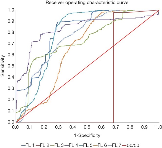
Best ROC curves. ROC curves for each feature list’s best performing correlation. FL 2 has the worst ROC curve with an AUC of 0.314. ROC, receiver operating characteristic; AUC, area under the ROC curve; FL, feature list.

Results of using positive features

Figures 6,7 show the heatmap and ROC curves for each FL using the positive features. As seen on the results summarized in Tables 2,3, there is no significant difference between the peak performing correlations for each feature transformation method and positive features with a change in average accuracy, HG accuracy, LG accuracy, and AUC of −0.065±0.059, −0.048±0.049, −0.083±0.080, and 0.061±0.123, respectively. However, using positive features significantly increased the ROC of FL 2 from 0.314 to 0.641. One explanation of the reduction of average accuracy in the positive features is the way that positive features were calculated. Positive features were calculated to be any added features that increased the overall accuracy of the classification over the full correlation limit range. However, the peak performances of many FLs were less than the full range of correlation limits tested, resulting in redundant or confounding features being added into the positive feature set as seen in Tables 2,3, reducing the performance slightly.

Figure 6.

Positive feature accuracy heatmap. A heatmap for each feature list using its positive features. Compared to Figure 4, the overall average accuracy, especially LG patients, suffers. HG, high-grade; LG, low-grade; FL, feature list.

Figure 7.

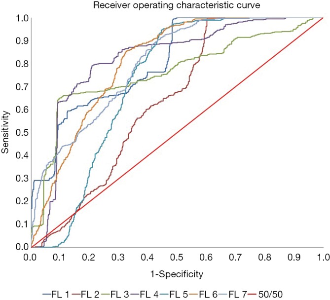
Positive feature ROC curves. Receiver operating characteristic curves for each feature list using its positive features. With positive features, the ROC of FL 2 significantly improves at the cost of some classification accuracy. ROC, receiver operating characteristic; FL, feature list.

Discussion

In our literature search, there were no studies we could make direct comparisons of our results. However, similar papers using DSC MRI or radiomic features to classify gliomas or GBMs were used to compare our method’s performance. Qin et al. (30) and Reza et al. (31) have shown that radiomic features on multiple MRI sequences could be used to grade gliomas and combined to achieve an AUC performance of 0.943 and 0.88 respectively. Our method is comparable to these state-of-the-art methods and could provide functional information such as calculated perfusion and permeability values (32) that could be applied to increase our accuracy.

One of the limitations of this work was the number of patients. Unfortunately, only a limited number of patients were available for the study within the inclusion criteria. Only 25 patients had FLAIR and DSC MRI images as well as having either biopsy or tumor resection with histopathological analysis. To alleviate the problems that comes with a small sample size, our study used a rigorous supervised feature selection to allow only significant features corresponding to the database. While making our study more robust to the small sample size, we are expecting and are planning to add more patients to this study as more data becomes available.

Out of the seven FLs, the FL with the best overall accuracy was FL 5 (82.12%), a normalized delta-radiomic FL. However, considering the disparity between HG and LG accuracies, we consider FL 4 (81%), a relative delta-radiomic feature method, to be better overall for its relatively high accuracy in both HG and LG patient classification. Moreover, by using the best-majority voting method, our method can take advantage of the differences in the seven FLs to achieve a better final result as seen in the increase from 0.821 to 0.902 and 0.797 to 0.938 for overall accuracy and AUC respectively.

When comparing FLs and the number of features used for each method, we observed that normalizing features to itself, especially through division (lists 2, 4, and 6), significantly reduced the number of features used for our classification method than their non-normalized counterparts. This is observed in lists 1 and 2 (71 vs. 24 features), lists 3 and 4 (522 vs. 87), and lists 5 and 6 (679 vs. 159). For each pair of FLs compared, overall performance parameters did not change significantly but reduced the number of features as well as computational load.

The most commonly used feature groups in all FLs are shown in Table 4. We can see that of the 69 features used in at least 4 feature transformation methods, 56 are gray-level-cooccurrence-matrix (GLCM), textural, features (30 derived from 2D slices and 26 from a 3D image matrix). Overwhelmingly, over 80% of the strong and common features used in our methods are textural features as described by Haralick et al. (33) in 1973 and later confirmed for the use in radiomic applications by Ravanelli et al. (34) in 2010 for non-small cell lung cancer (NSCLC) and Aerts et al. (13) in 2014 for a more general application. These commonly used features may be the radiomic signature, or finger print, for classifications of GBMs using DSC MRI data and could allow future studies to test with and against these features to develop a robust classification or predictive model.

Table 4. Table of commonly used features and feature groups.

Number of lists used	Feature groups	Feature
6 feature lists	GLCM (2D)	InverseVariance [2]
	GLCM (3D)	InverseVariance [1]
5 feature lists	GLCM (2D)	InformationMeasureCorr2 [2]
		InverseVariance [6]
		MaxProbability [2]
	GLCM (3D)	Correlation [1]
		InverseVariance [3]
	Intensity direct	60Percentile [1]
	Intensity histogram	5PercentileArea [1]
4 feature lists	GLCM (2D)	Contrast [2]
		Correlation [7]
		InformationMeasureCorr1 [2]
		InformationMeasureCorr2 [1]
		InverseDiffMomentNorm [1]
		InverseVariance [1]
		MaxProbability [4]
	GLCM (3D)	ClusterProminence [2]
		Contrast [2]
		Correlation [6]
		Homogeneity2 [2]
		InverseVariance [4]
		MaxProbability [4]
		SumEntropy [1]
	GLRLM (2D)	HighGrayLevelRunEmpha [1]
	Intensity direct	GlobalMax [1]
		LocalStdMedian [1]
		5Percentile [1]
		Range [1]
	Intensity histogram	5Percentile [1]
		60Percentile [1]
		Range [1]
	Neighbor intensity difference (2D)	TextureStrength [1]
	Neighbor intensity difference (3D)	Contrast [1]

GLCM, gray-level-cooccurrence-matrix; GLRLM, gray-level run length matrix.

Adding time and/or sequential information as features were considered as well. However, those features were not included in this study for the following reasons: (I) sequential features would be eliminated during the t-test of the feature selection process since there are no significant differences in the sequential order of DSC MRIs based on patient GBM grade; (II) time information would be arbitrary based on when the MRI was taken and also eliminated during the t-test for significance between the high and LG patients. In future studies, our method should involve either multi-class labeling or require a feature selection method that preserves the sequential and time information.

Conclusions

In conclusion, our method using delta-radiomic features of DSC MRI performed well in classifying HG and LG GBMs based on the DSC MRI data with an average of 90% accuracy. This study shows that delta-radiomic features of DSC MRI, specifically GLCM and other textural features, are highly correlated with tumor grades that may further elucidate the underlying tumor biology and response to therapy. The radiomic analysis assisted by machine learning as demonstrated in this study can be generalized to a broader set of diseases and imaging modalities. Our method derived several delta-radiomic features using the difference in DCS MRI between the normal and disease tissue as well as the change in features from the baseline. However, it is the combination of these features and reducing individual biases that gave us the best results. This method will be tested further as more patients are included and clinical outcome information becomes available such as testing our method’s ability to stratify even LG gliomas. With future advances in imaging, machine learning, and radiomic analysis, a more robust, accurate and validated classification or predictive model will be widely available to assist future oncologists deliver better and more personalized treatments.

Ethical Statement: The use of these MRI data was approved by the Emory institutional review board (IRB) with written informed consent obtained from the study subjects.

References

- 1.Surawicz TS, McCarthy BJ, Kupelian V, Jukich PJ, Bruner JM, Davis FG. Descriptive epidemiology of primary brain and CNS tumors: results from the Central Brain Tumor Registry of the United States, 1990-1994. Neuro Oncol 1999;1:14-25. 10.1093/neuonc/1.1.14 [DOI] [PMC free article] [PubMed] [Google Scholar]
- 2.Shapiro WR, Green SB, Burger PC, Mahaley MS, Jr, Selker RG, VanGilder JC, Robertson JT, Ransohoff J, Mealey J, Jr, Strike TA, Pistenmaa DA. Randomized trial of three chemotherapy regimens and two radiotherapy regimens and two radiotherapy regimens in postoperative treatment of malignant glioma. Brain Tumor Cooperative Group Trial 8001. J Neurosurg 1989;71:1-9. 10.3171/jns.1989.71.1.0001 [DOI] [PubMed] [Google Scholar]
- 3.Narang S, Lehrer M, Yang D, Lee J, Rao A. Radiomics in glioblastoma: current status, challenges and potential opportunities. Transl Cancer Res 2016;5:383-97. 10.21037/tcr.2016.06.31 [DOI] [Google Scholar]
- 4.Weber RG, Sabel M, Reifenberger J, Sommer C, Oberstrass J, Reifenberger G, Kiessling M, Cremer T. Characterization of genomic alterations associated with glioma progression by comparative genomic hybridization. Oncogene 1996;13:983-94. [PubMed] [Google Scholar]
- 5.Brennan CW, Verhaak RG, McKenna A, Campos B, Noushmehr H, Salama SR, Zheng S, Chakravarty D, Sanborn JZ, Berman SH, Beroukhim R, Bernard B, Wu CJ, Genovese G, Shmulevich I, Barnholtz-Sloan J, Zou L, Vegesna R, Shukla SA, Ciriello G, Yung WK, Zhang W, Sougnez C, Mikkelsen T, Aldape K, Bigner DD, Van Meir EG, Prados M, Sloan A, Black KL, Eschbacher J, Finocchiaro G, Friedman W, Andrews DW, Guha A, Iacocca M, O'Neill BP, Foltz G, Myers J, Weisenberger DJ, Penny R, Kucherlapati R, Perou CM, Hayes DN, Gibbs R, Marra M, Mills GB, Lander E, Spellman P, Wilson R, Sander C, Weinstein J, Meyerson M, Gabriel S, Laird PW, Haussler D, Getz G, Chin L, Network TR. The somatic genomic landscape of glioblastoma. Cell 2013;155:462-77. 10.1016/j.cell.2013.09.034 [DOI] [PMC free article] [PubMed] [Google Scholar]
- 6.Nobusawa S, Watanabe T, Kleihues P, Ohgaki H. IDH1 mutations as molecular signature and predictive factor of secondary glioblastomas. Clin Cancer Res 2009;15:6002-7. 10.1158/1078-0432.CCR-09-0715 [DOI] [PubMed] [Google Scholar]
- 7.Hartmann C, Hentschel B, Wick W, Capper D, Felsberg J, Simon M, Westphal M, Schackert G, Meyermann R, Pietsch T, Reifenberger G, Weller M, Loeffler M, von Deimling A. Patients with IDH1 wild type anaplastic astrocytomas exhibit worse prognosis than IDH1-mutated glioblastomas, and IDH1 mutation status accounts for the unfavorable prognostic effect of higher age: implications for classification of gliomas. Acta Neuropathol 2010;120:707-18. 10.1007/s00401-010-0781-z [DOI] [PubMed] [Google Scholar]
- 8.Verhaak RG, Hoadley KA, Purdom E, Wang V, Qi Y, Wilkerson MD, Miller CR, Ding L, Golub T, Mesirov JP, Alexe G, Lawrence M, O'Kelly M, Tamayo P, Weir BA, Gabriel S, Winckler W, Gupta S, Jakkula L, Feiler HS, Hodgson JG, James CD, Sarkaria JN, Brennan C, Kahn A, Spellman PT, Wilson RK, Speed TP, Gray JW, Meyerson M, Getz G, Perou CM, Hayes DN, Cancer Genome Atlas Research Network Integrated genomic analysis identifies clinically relevant subtypes of glioblastoma characterized by abnormalities in PDGFRA, IDH1, EGFR, and NF1. Cancer Cell 2010;17:98-110. 10.1016/j.ccr.2009.12.020 [DOI] [PMC free article] [PubMed] [Google Scholar]
- 9.Patel AP, Tirosh I, Trombetta JJ, Shalek AK, Gillespie SM, Wakimoto H, Cahill DP, Nahed BV, Curry WT, Martuza RL, Louis DN, Rozenblatt-Rosen O, Suva ML, Regev A, Bernstein BE. Single-cell RNA-seq highlights intratumoral heterogeneity in primary glioblastoma. Science 2014;344:1396-401. 10.1126/science.1254257 [DOI] [PMC free article] [PubMed] [Google Scholar]
- 10.Parker NR, Khong P, Parkinson JF, Howell VM, Wheeler HR. Molecular heterogeneity in glioblastoma: potential clinical implications. Front Oncol 2015;5:55. 10.3389/fonc.2015.00055 [DOI] [PMC free article] [PubMed] [Google Scholar]
- 11.Sottoriva A, Spiteri I, Piccirillo SG, Touloumis A, Collins VP, Marioni JC, Curtis C, Watts C, Tavare S. Intratumor heterogeneity in human glioblastoma reflects cancer evolutionary dynamics. Proc Natl Acad Sci U S A 2013;110:4009-14. 10.1073/pnas.1219747110 [DOI] [PMC free article] [PubMed] [Google Scholar]
- 12.Moton S, Elbanan M, Zinn PO, Colen RR. Imaging Genomics of Glioblastoma: Biology, Biomarkers, and Breakthroughs. Top Magn Reson Imaging 2015;24:155-63. 10.1097/RMR.0000000000000052 [DOI] [PubMed] [Google Scholar]
- 13.Aerts HJ, Velazquez ER, Leijenaar RT, Parmar C, Grossmann P, Carvalho S, Bussink J, Monshouwer R, Haibe-Kains B, Rietveld D, Hoebers F, Rietbergen MM, Leemans CR, Dekker A, Quackenbush J, Gillies RJ, Lambin P. Decoding tumour phenotype by noninvasive imaging using a quantitative radiomics approach. Nat Commun 2014;5:4006. 10.1038/ncomms5006 [DOI] [PMC free article] [PubMed] [Google Scholar]
- 14.Yang X, Tridandapani S, Beitler JJ, Yu DS, Yoshida EJ, Curran WJ, Liu T. Ultrasound GLCM texture analysis of radiation-induced parotid-gland injury in head-and-neck cancer radiotherapy: an in vivo study of late toxicity. Med Phys 2012;39:5732-9. 10.1118/1.4747526 [DOI] [PMC free article] [PubMed] [Google Scholar]
- 15.Yamamoto S, Maki DD, Korn RL, Kuo MD. Radiogenomic analysis of breast cancer using MRI: a preliminary study to define the landscape. AJR Am J Roentgenol 2012;199:654-63. 10.2214/AJR.11.7824 [DOI] [PubMed] [Google Scholar]
- 16.Lee J, Narang S, Martinez JJ, Rao G, Rao A. Associating spatial diversity features of radiologically defined tumor habitats with epidermal growth factor receptor driver status and 12-month survival in glioblastoma: methods and preliminary investigation. J Med Imaging (Bellingham) 2015;2:041006. 10.1117/1.JMI.2.4.041006 [DOI] [PMC free article] [PubMed] [Google Scholar]
- 17.Hatt M, Majdoub M, Vallieres M, Tixier F, Le Rest CC, Groheux D, Hindie E, Martineau A, Pradier O, Hustinx R, Perdrisot R, Guillevin R, El Naqa I, Visvikis D. 18F-FDG PET uptake characterization through texture analysis: investigating the complementary nature of heterogeneity and functional tumor volume in a multi-cancer site patient cohort. J Nucl Med 2015;56:38-44. 10.2967/jnumed.114.144055 [DOI] [PubMed] [Google Scholar]
- 18.Liu Y, Shi X, Xia Y, Lei Y, Tang L, Liu T, Curran W, Mao H, Yang X. Multi-Scale V-Net: A Deep Learning Framework for Brain Tumor Segmentation in Multiparametric MRI. Med Phys 2018;45:E568. [Google Scholar]
- 19.Zhang L, Fried DV, Fave XJ, Hunter LA, Yang J, Court LE. IBEX: an open infrastructure software platform to facilitate collaborative work in radiomics. Med Phys 2015;42:1341-53. 10.1118/1.4908210 [DOI] [PMC free article] [PubMed] [Google Scholar]
- 20.Nanni L, Ghidoni S, Brahnam S. Handcrafted vs. non-handcrafted features for computer vision classification. Pattern Recognit 2017;71:158-72. 10.1016/j.patcog.2017.05.025 [DOI] [Google Scholar]
- 21.Lei Y, Tang X, Higgins K, Lin J, Jeong J, Liu T, Dhabaan A, Wang T, Dong X, Press R, Curran WJ, Yang X. Learning-based CBCT correction using alternating random forest based on auto-context model. Med Phys 2019;46:601-18. [DOI] [PMC free article] [PubMed] [Google Scholar]
- 22.Lei Y, Jeong JJ, Wang T, Shu HK, Patel P, Tian S, Liu T, Shim H, Mao H, Jani AB, Curran WJ, Yang X. MRI-based pseudo CT synthesis using anatomical signature and alternating random forest with iterative refinement model. J Med Imaging (Bellingham) 2018;5:043504. 10.1117/1.JMI.5.4.043504 [DOI] [PMC free article] [PubMed] [Google Scholar]
- 23.Yang XF, Lei Y, Shu HK, Rossi P, Mao H, Shim H, Curran WJ, Liu T. Pseudo CT Estimation from MRI Using Patch-based Random Forest. Medical Imaging 2017: Image Processing 2017;10133. [DOI] [PMC free article] [PubMed]
- 24.Yang X, Lei Y, Higgins K, Wang T, Tian S, Dhabaan A, Shim H, Mao H, Curran W, Shu H, Liu T. Patient-Specific Pseudo-CT Generation Using Semantic and Contextual Information-Based Random Forest for MRI-Only Radiation Treatment Planning. Med Phys 2018;45:E702. [Google Scholar]
- 25.Lei Y, Harms J, Wang T, Tian S, Zhou J, Shu HK, Zhong J, Mao H, Curran WJ, Liu T, Yang X. MRI-based synthetic CT generation using semantic random forest with iterative refinement. Phys Med Biol 2019;64:085001. 10.1088/1361-6560/ab0b66 [DOI] [PMC free article] [PubMed] [Google Scholar]
- 26.Lei Y, Wang T, Harms J, Shafai-Erfani G, Tian S, Higgins K, Shu HK, Shim H, Mao H, Curran WJ, Liu T, Yang X. MRI-based pseudo CT generation using classification and regression random forest. SPIE Medical Imaging, San Diego, California, United States, 2019. doi: 10.1117/12.2512560 [DOI] [Google Scholar]
- 27.Breiman L. Random Forests. Machine Learning 2001;45:5-32. 10.1023/A:1010933404324 [DOI] [Google Scholar]
- 28.Hastie T, Tibshirani R, Friedman J. The Elements of Statistical Learning: Data Mining, Inference, and Prediction. 2nd edition. Springer-Verlag New York, 2009. [Google Scholar]
- 29.Wesseling P, Kros JM, Jeuken JW. The pathological diagnosis of diffuse gliomas: towards a smart synthesis of microscopic and molecular information in a multidisciplinary context. Diagn Histopathol (Oxf) 2011;17:486-94. 10.1016/j.mpdhp.2011.08.005 [DOI] [Google Scholar]
- 30.Qin JB, Liu Z, Zhang H, Shen C, Wang XC, Tan Y, Wang S, Wu XF, Tian J. Grading of Gliomas by Using Radiomic Features on Multiple Magnetic Resonance Imaging (MRI) Sequences. Med Sci Monit 2017;23:2168-78. 10.12659/MSM.901270 [DOI] [PMC free article] [PubMed] [Google Scholar]
- 31.Reza SMS, Samad MD, Shboul ZA, Jones KA, Iftekharuddin KM. Glioma grading using structural magnetic resonance imaging and molecular data. J Med Imaging (Bellingham) 2019;6:024501. 10.1117/1.JMI.6.2.024501 [DOI] [PMC free article] [PubMed] [Google Scholar]
- 32.Artzi M, Blumenthal DT, Bokstein F, Nadav G, Liberman G, Aizenstein O, Ben Bashat D. Classification of tumor area using combined DCE and DSC MRI in patients with glioblastoma. J Neurooncol 2015;121:349-57. 10.1007/s11060-014-1639-3 [DOI] [PubMed] [Google Scholar]
- 33.Haralick RM, Shanmugam K, Dinstein I. Textural Features for Image Classification. IEEE Transactions on Systems, Man, and Cybernetics 1973;SMC-3:610-21. 10.1109/TSMC.1973.4309314 [DOI] [Google Scholar]
- 34.Ravanelli M, Farina D, Morassi M, Roca E, Cavalleri G, Tassi G, Maroldi R. Texture analysis of advanced non-small cell lung cancer (NSCLC) on contrast-enhanced computed tomography: prediction of the response to the first-line chemotherapy. Eur Radiol 2013;23:3450-5. 10.1007/s00330-013-2965-0 [DOI] [PubMed] [Google Scholar]