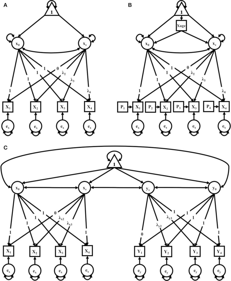
FIGURE 1 |.
(A–C) path diagrams for Clusters 1–3. Path diagrams are visual representations of model parameters and their relationships, in which each type of model parameter is provided a graphical symbol, i.e., squares or rectangles are used for observed variables (i.e., indicators), circles are used for latent variables and error terms, straight arrows for hypothetical causal or direct effects, and curved arrows for covariances (Kline, 2016). In all path diagrams presented here (A–C), composite scores of pub-directed behaviors (PDBs) for each litter (1–4) are represented as sequential squares (from left to right) around indicators by Xt or Yt, where t = litter. Each represented composite score (e.g., Xt or Yt) has an error term, ex or ey, which represents variance not explained by the composite scores, including variance due to measurement error. Elements of regression, intercept and slope, are represented by x0 and xs, respectively, and circumscribed to represent their status as latent variables, each with their own covariance and a covariance between the two. Triangles containing the number 1 represent the inclusion of a term for the analysis of means. As the intercept for each model does not change across time, straight arrows from the intercept factor to each time point are labeled with the number 1, indicating a constraint on estimation of the regression between the intercept and each time point. Straight arrows from the slope factor (xs or ys) are variably constrained, according to the growth pattern in consideration. Thus, for the no growth model, regression paths from the slope factor to indicators at all time points are constrained to 0; for the linear growth model, regression paths from the slope factor to indicators are constrained to 0, .33, .67, and 1 for litters 1, 2, 3, and 4, respectively; and for the non-linear growth model, only the regression path from the slope factor to litter 1 is constrained (to 0) and all others are freely estimated, as represented by the term λt. Path diagram (A) represents models tested in Cluster 1, the Independent Maternal and Paternal Models, which includes only the common parameters outlined above. Path diagram (B) represents models tested in Cluster 2, the Independent Maternal and Paternal Models with Covariates, which expands upon the model given for Cluster 1 with the addition of a time-invariant covariate for parental age (Xage) and time-varying covariates for litter size (Pt), both given in squares. Path diagram (C) represents models tested in Cluster 3, the Maternal-Paternal Bivariate Model, which expands upon the model given for Cluster 1 by presenting models for change in maternal and paternal care in parallel with double headed arrows representing covariance between the two models, and therefore covarying trajectories of change between mothers and fathers.

