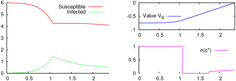
Figure 11:
An example time-series plot of the equilibrium trajectory to the finite-horizon problem calculated with S(0) = 6, I(0) = 0.01, m = 2, and T = 2.37. Panels show the state-variables S(t) and I(t) (left), along with the price of susceptibility VS(t) (top right), and the relative contact rate σ(c*) under the equilibrium control c*(t) (bottom right). In this case, 0 < t1 < t2 < t3 = T.

