Figure 1. Kymograph generation and KymoButler.

Figure 1—figure supplement 1. Example kymographs and software workflow.

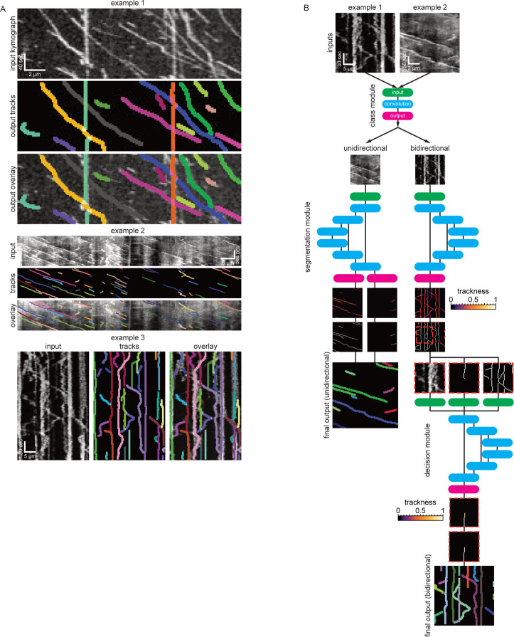
(A) Three example kymographs from published manuscripts. Example 1: In vitro dynamics of single cytoplasmic dynein proteins adapted from Tanenbaum et al. (2013). Example 2: EB1-GFP labelled growing microtubule plus-ends in mouse dorsal root ganglion axons (Lazarus et al., 2013). Example 3: Mitochondria dynamics in mouse retinal ganglion cell dendrites (Faits et al., 2016). Each dilated coloured line depicts an identified track. (B) KymoButler software workflow. First, a classification module is applied to each kymograph to determine whether the kymograph is unidirectional or bidirectional. If the kymograph is deemed unidirectional the unidirectional segmentation module is applied to the image to generate two trackness maps that assign each pixel a score between 0–1, approximating the likelihood that this pixel is part of a track with negative slope (left image) or positive slope (right image). Subsequently, the trackness maps are binarized, skeletonised, and segmented into their respective connected components. Finally, those components are averaged over each row to generate individual tracks, and a dilated representation of each track is plotted in a random colour. If the kymograph is classified as bidirectional, another segmentation module is applied to the kymograph, which generates a trackness map that does not highlight any particular slope. This map is binarized with a user-defined threshold and subsequently skeletonised, resulting in a binary map that exhibits multiple track crossings. To resolve these crossings, we first apply a morphological operation that detects the starting points of tracks in the binary map (red dots). Then, the algorithm tracks each line from its starting point until a crossing is encountered. At each crossing, the decision module is called, whose inputs are (i) the raw kymograph in that region, (ii) the previous track skeleton, and (iii) all possible tracks in that region. The decision module then generates another trackness map that assigns high values to the most likely future path from the crossing. This map is then again binarized and thinned with a fixed threshold of 0.5. If the predicted path is longer than two pixels, the path tracking continues. Once all starting points have been tracked until an end (either no prediction or no further pixels available), the algorithm again looks for starting points in the skeletonised trackness map excluding the identified tracks, and repeats the steps outlined above until all pixels are occupied by a track. The resulting tracks are then drawn with each track in a random colour.

Figure 1—figure supplement 2. The software modules in detail.

(A) The class module. This module resizes any input kymograph to 64 × 64 pixels. It subsequently applies two convBlocks with no padding and 64 output feature maps to the image. ConvBlocks comprise a convolutional layer with 3 × 3 kernels followed by a BatchNormalisation Layer and a leaky Rectified Linear Unit (ReLU) activation function (leak factor 0.1). The convBlocks are followed by 2 × 2 max pooling to halve the feature map sizes. This is repeated another two times while steadily increasing the number of feature maps until the last convBlock generates 256 feature maps of size 9 × 9. These maps are then pooled with a final 2 × 2 max pool operation followed by a 4 × 4 mean pool operation to generate a vector of 256 features. These features are then classified with a fully connected layer with output nodes followed by another leaky Ramp and finally another fully connected layer generates two output values that correspond to the probability of being a unidirectional/bidirectional kymograph. (B) The unidirectional segmentation module takes and an input kymograph of arbitrary size. Subsequently two convBlocks with 64 output feature maps are applied to the image followed by max pooling. This is repeated three times while doubling the number of feature maps with each pooling operation forming the ‘contracting path’. To obtain an image of the same size as the input image the small feature maps at the lowest level of the network have to be deconvolved four times each time halving the number of feature maps and applying further convBlocks. After each 2 × 2 deconvolution the resulting feature maps are catenated with the feature maps of the same size from the contracting path so that the network only learns residual alterations of the input image. The final 64 feature maps are linked to two independent convolutional layers that generate outputs that correspond to the trackness scores for positive and negative sloped lines. (C) The bidirectional segmentation module has the same architecture as the unidirectional one but only generates one output that corresponds to the trackness map for any lines in the image. (D) The decision module architecture is the same as the bidirectional segmentation module but takes three input images instead of one.

Figure 1—figure supplement 3. Synthetic training data examples.

(A) Class module training data consisted of 64 × 64 pixel images that were either classified as unidirectional (example 1) or bidirectional (example 2). (B) Synthetic training data for the unidirectional segmentation module comprised 300 × 300 pixel kymographs with two binary ground truth maps, corresponding to particle motion with negative and positive slopes. (C) Synthetic bidirectional segmentation module training data comprises 300 × 300 pixel kymographs with only one ground truth image containing all ground truth tracks. (D) The decision module was trained with 48 × 48 pixel image crops of the raw kymograph, the previous skeletonised path, and all the skeletonised paths in the cropped region. The ground truth is simply the known future segment of the given path.

Figure 1—figure supplement 4. Geometric mean of track recall and precision for different trackness thresholds.

(A) 10 synthetic unidirectional and bidirectional kymographs were analysed with varying trackness thresholds, and track recall and track precision were calculated. The geometric mean of recall and precision does not exhibit much variation between 0.1 and 0.3 but decreases at lower and higher values. Individual dots represent per kymograph values and the solid lines the binned mean.

Figure 1—figure supplement 5. Geometric mean of track recall and precision for different signal to noise ratios and particle densities.

(A, B) The same synthetic (A) bidirectional and (B) unidirectional kymograph for three different SNR values (top). Note that some tracks become almost invisible at low SNRs. Bottom: Overlay of the tracks predicted by KymoButler (magenta, not post processed) with the ground truth (green). (C) A low SNR unidirectional/bidirectional kymograph analysed by KymoButler and manual annotation. Predicted tracks in magenta and ground truth in green. (D) The geometric mean of track recall and precision as a function of SNR. The same 10 kymographs were noised with different SNRs and the average score taken. Dots represent individual kymographs and the line the 0.1 bin average. Highlighted dots represent manually analysed kymographs. (E, F) Three example (E) bidirectional and (F) unidirectional kymographs for different particle densities (top). The percentage value gives the percentage of the image covered with signal. Bottom: Overlay of the tracks predicted by KymoButler (magenta) with the ground truth (green). (G) A high particle density unidirectional/bidirectional kymograph analysed with KymoButler and manual annotation. Predicted tracks in magenta and ground truth in green. (H) The geometric mean of track recall and precision as a function of coverage percentage. 20 kymographs were generated with varying numbers of particles. Tracks smaller than three pixels and shorter than three frames were discarded for unidirectional kymograph quantification while tracks smaller than 10 pixels and shorter than 25 frames were discarded for bidirectional kymograph quantification. Dots represent individual kymographs and the line the 5% bin average. Highlighted dots represent manually analysed kymographs.