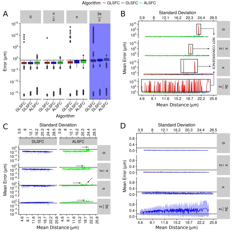
Appendix 1—figure 5. Error in the adjustment of the algorithms DLSFC, GLSFC and ALSFC.

The error was quantified through Equation (21). In all panels, the horizontal black line represents the value $y=0.1732\mu m$ (see Equation (21)). (A) Boxplot of the error distribution for each algorithm taking into account the partial occlusion angles (four sub-panels). The x-axis specifies the name of the algorithm and the y-axis the error in microns. The blue shadow in the sub-panel ${\displaystyle \frac{3\pi }{2}}$ represents the occlusion angle in which the mean value of the errors are greater than $0.1732\mu m$. (B) Mean error of the adjustment by the algorithms DLSFC, GLSFC and ALSFC. The bottom x-axis is the Mean distance of the corrupted points to the ‘ground truth’ circumference (see Equation (20)), and the up x-axis is the Standard Deviation. The figure is split out in four sub-panels in accordance with the occlusion angle. The black boxes show examples in which the algorithm GLSFC does not reach the convergence (extremely high error). The arrows mark out some examples where the algorithm ALSFC does not have have a good adjustment. (C) Zoom of the performance of the algorithms DLSFC and ALSFC. (D) Results of the algorithm DLSFC. The graphics in the panel (C)) and (D)) also shows the confidence interval around the mean (see green and blue shadows), it was computed as $\overline{d_{𝒞}}\pm \sigma (d_{𝒞})$.