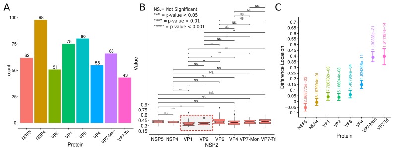
Appendix 1—figure 7. Supplementary exploratory analysis of the results obtained by the algorithm VPs-DLSFC.

(A) Histogram with the numbers of VPs that were obtained as part of the pre-segmentation step of the algorithm described in Appendix 1—figure 1A. Note that because each image contains one and only one VP, this histogram represents also the numbers of pre-segmented images that we had in our study. (B) Graphical representation of the Mann-Whitney hypothesis test in two-by-two comparison between the radii distributions of NSP2 in each experiment (Mann and Whitney, 1947). To avoid confusions, for each box, under the NSP2 name in x-axis, we included the name of the accompanying protein that specifies in which experiment we obtain that distribution of NSP2. Each combination is linked by a line, and the result of the test is up of the line. The red dashed square highlights the only two combinations (VP1 and VP2) in which the distribution of NSP2 had a significant statistical difference with the other NSP2 distributions. (C) Two-sample Mann-Whitney hypothesis test, considering as variables the radius of NSP2 in contrast to the radius of the others seven proteins. In each combination, we show the difference in location between NSP2 and the other protein (x-axis) and the confidence interval at a level of 95%. The numbers over the intervals confidence are the p-value of the statistical test.