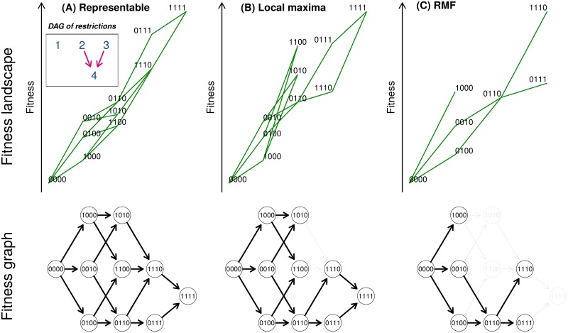
Fig 1. Fitness landscapes, paths of tumor progression, and directed acyclic graphs (DAGs) of restrictions in the order of accumulation of mutations for the three types of landscapes used.

(A) Representable; (B) Local maxima; (C) Rough Mount Fuji (RMF). Top row: partial fitness landscapes (representation based on [23], but only accessible genotypes are shown); genotypes are shown as sequences of 0s and 1s, where “1010” means a genotype with the first and third driver genes mutated; the vertical position of a genotype is its fitness; its horizontal position on the x-axis is given by its Hamming distance to the “0000” genotype. Green segments connect mutational neighbors of increasing fitness. The inset in the first row shows the DAG of restrictions in the order of accumulation of mutations that applies to (A) and (B). A DAG of restrictions shows genes (not genotypes) in the nodes; an arrow from gene i to gene j means that a mutation in i must occur before a mutation in j can occur; an arrow indicates a direct dependency of a mutation in gene j on a mutation in gene i. In the figure, a mutation in the fourth gene can be observed only if both the second and third genes are mutated. Note that among the models considered in this paper, CAPRESE and OT can only represent trees (so they can not account for the fourth gene having two, or more, incoming arrows). The absence of an arrow between two genes means that there are no direct dependencies between the two genes. Bottom row: fitness graphs or graphs of mutational paths; in fitness graphs nodes are genotypes and arrows point toward mutational neighbors of higher fitness (i.e., two genotypes connected by an arrow differ in one mutation that increases fitness [24–26]). These fitness graphs show all the paths of tumor progression, the set of accessible mutational paths and adaptive walks that, under the restriction that there can be no back mutations, start from the “0000” genotype and end in a fitness maximum. When evolution runs until fixation in a fitness maximum, each path from “0000” to a fitness maximum corresponds to a different Line of Descent (LOD). For (B) and (C), gray edges and nodes in the fitness graphs show edges and nodes that are present in (A) but missing in (B) or (C). Under CPMs, since each new driver mutation with its dependencies satisfied increases fitness, all accessible genotypes that differ by exactly one mutation are connected in the fitness graph, as shown in (A), and the genotype with all driver genes mutated is the single fitness maximum (see also section 4 of S2 Text for local maxima from unconditionally deleterious mutations). For (B), the fitness landscape —and its fitness graph— has the same accessible genotypes as the fitness landscape in (A). But the fitness landscape in (B) has three maxima and, compared to (A), there are fewer paths to the genotype with all genes mutated, “1111”, and several paths end in the other two maxima (“1100”, “1010”). Thus, the fitness graph of (B) does not fulfill the assumptions of CPMs. Compared to the fitness graph of (A), in the fitness graph of (B) not all accessible genotypes that differ by one mutation are connected —e.g., genotypes “1100” and “1110”. In terms of acquisition of mutations, in (B), and in contrast to (A), we cannot reach genotype “1110” from genotype “1100”, even when a mutation in the third gene does not depend on any previous mutation according to the DAG of restrictions. So if we go from “1000” to “1100”, the acquisition of the second mutation precludes acquiring the third mutation (a violation of an assumption of CPMs), and this creates a local fitness maximum. The fitness landscape in (C) cannot be represented by any DAG of restrictions: no DAG of restrictions can account at the same time for the presence of genotypes “1000”, “0100”, “0010”, and the absence of every double mutant with the first gene mutated. Relative to (A), the fitness graph in (C) is missing both paths and genotypes (relative to the fitness graph from any possible DAG of restrictions it could either be missing and/or adding genotypes and paths).