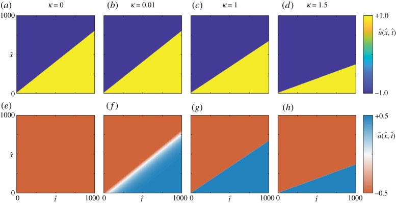
Figure 3.

The solution to the continuous model, equation (2.6), shown as kymographs where colouring represents (a–d) the displacement function, $\hat{u}(\hat{x},\hat{t})$, and (e–h) the biological response, $\hat{a}(\hat{x},\hat{t})$, for increasing values of κ. Parameter values used are ν = 4 and η = 2. Each signal is initiated using the initial condition described by equations (2.8) and (2.9) with Q = 1. (Online version in colour.)