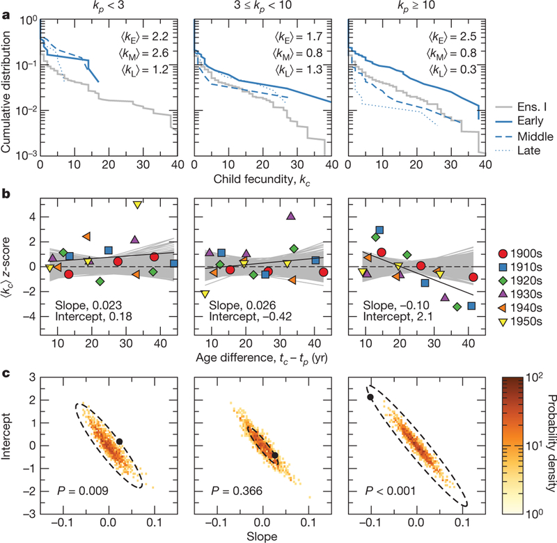
Figure 4 |. Effect of age difference between mentor and protégé, t_c − t_p, on protégé fecundity.

a, Fecundity distribution of children born during the 1910s (for which the average fecundity was 1.4) to parents with k_p < 3, 3 ≤ k_p < 10 and k_p ≥ 10, compared with the expectation from ensemble I (grey line). We separate children into terciles (early, middle, late) according to t_c − t_p, and denote the average fecundities of the children born early, middle and late in their parents’ lives as $\langle k_{\text{E}}\rangle$, $\langle k_{\text{M}}\rangle$ and $\langle k_{\text{L}}\rangle$, respectively. The average fecundity of children born to parents with k_p < 3 is higher than expected, regardless of whether they were born during the early, middle or later part of their parents’ lives. We also note that the average fecundity of children born to parents with k_p ≥ 10 decreases throughout their parents’ lives. b, We quantify the significance of these trends during each decade (coloured symbols) by computing the z-score of the average child fecundity, $\langle k_c\rangle$, compared with the average child fecundity in networks from ensemble I. This information is summarized by identifying the linear regression (solid black line; slope and intercept as shown). The regression lines for networks from our null model (grey lines) vary around the expectation of our null model (dashed black line). c, Significance of linear regressions in b. We compare the slope and intercept of the empirical regression (black circle) with the distribution of the slope and intercept of the same quantities computed from the null model. Because these quantities are approximately distributed as a multivariate Gaussian, we compute the equivalent of a two-tailed P value by finding the fraction of synthetically generated slope–intercept pairs that lie outside the equiprobability surface of the multivariate Gaussian (dashed ellipse). The slopes and intercepts of the regressions for children of parents with low (P = 0.009) and high (P < 0.001) fecundities are significantly different from the expectations for the null model, consistent with the data displayed in a. Comparisons with expectations from random networks from ensemble II yield the same conclusions (Supplementary Fig. 4).