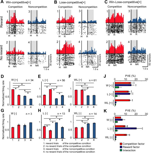
Figure 3.
LPFC neurons that showed competitive activities. A–C, Raster and histogram displays for neurons that showed competitive activities: Win-competitive[+] (A), Lose-competitive[+] (B), and Win–Lose-competitive[+] (C). Displays in the left and right columns show activity in the competitive and noncompetitive conditions, respectively. The top and bottom rows show activity during reward and no-reward trials, respectively. The left vertical line in each display indicates the timing of a successful hit by either monkey. The right vertical line indicates the timing of a reward delivery (reward trials) or 1 s after a successful hit (no-reward trials). Each shaded area indicates the period when the typical activity of each type was observed. H, Successful hit; R, reward delivery; NR, 1 s after a successful hit. D–I, Mean relative magnitude of activity calculated from population data for each type of neuron (normalized mean ± SEM). D, Win-competitive[+]; E, Lose-competitive[+]; F, Win–Lose-competitive[+]; G, Win-competitive[−]; H, Lose-competitive[−]; and I, Win–Lose-competitive[−]. To obtain normalized population activity, we first obtained the mean spike rates for each neuron. We then calculated the relative magnitude of the spike rate for each type of neuron by alignment of the type of neuron in which the highest activity was observed. This analysis was conducted for the period in which the effect size was larger for each neuron. Data from different analysis periods were pooled and averaged. The mean relative magnitudes were significantly different among trial types for all types of neurons (Kruskal–Wallis H test, Win-competitive[+], H = 90.46, p < 10−19; Lose-competitive[+], H = 153.61, p < 10−33; Win–Lose-competitive[+], H = 176.18, p < 10−38; Win-competitive[−], H = 8.87, p = 0.03; Lose-competitive[−], H = 37.5, p < 10−8; Win–Lose-competitive[−], H = 38.95, p < 10−8). *p < 0.05, Bonferroni's-corrected two-tailed Mann–Whitney U test. W[+], Win-competitive[+]; L[+], Lose-competitive[+]; WL[+], Win–Lose-competitive[+]; W[−], Win-competitive[−]; L[−], Lose-competitive[−]; WL[−], Win–Lose-competitive[−]. J, K, Mean PVE. The plot shows the averaged PVE of each factor in the two-way ANCOVA (competition and reward factors and their interaction), separately for each type of neuron (mean ± SEM). We used a two-tailed Mann–Whitney U test to determine whether these PVE values were significantly greater than the chance level by comparing them with those calculated from the randomized data. *p < 0.05; **p < 10−5.

