Figure 4.

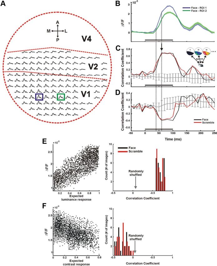
Spatial correlation between the maps of the population response and the expected response. A, Neural response time course along the imaged cortical space evoked by a face stimulus. Each plot corresponds to the mean signal averaged over 1 × 1 mm² (6 × 6 pixels). Dashed red lines schematically mark borders between cortical regions. B, Enlargement of the signals averaged over the region of interest (ROI) in the blue and green boxes in B. Trace width denotes ±1 SEM over 28 trials; the black bar represents the stimulus presentation time. C, D, Typical example of spatial correlation between the neural response (spread over 2034 pixels in V1) and cortical mapping of the expected luminance response (C) and the expected contrast response (D) as a function of time (see Materials and Methods). Black and red lines correspond to a coherent face stimulus (shown in A and B) and a scramble stimulus, respectively. Gray curve, correlation between the measured neural activity and the expected activity computed on a randomly shuffled set of stimuli (mean ± SD, n = 50). Dashed gray lines, the first time point exhibiting significant correlation and the time point with maximal correlation. Black bar denotes stimulus presentation. E, Left, Shows an example of a scatter plot of the expected luminance response of one face stimulus versus the neural response of all the pixels in V1 during one frame (t = 60 ms after stimulus onset, marked with an arrow in D, r = 0.69). Right, Shows the histogram of the spatial correlation values of all the images presented to both monkeys (n_face = 26, n_scramble = 26, scrambled images include both types of scrambling) at t = 60 ms after stimulus onset. No significant difference was found between the face and scramble. F, Same as in E, only for the correlation between the expected contrast response and the neural response (r = −0.39).