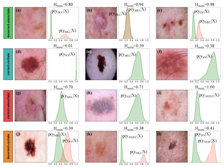
Figure 5.

Illustrating sample output posterior distributions and the corresponding uncertainty estimates using the Bayesian DenseNet-169. The Bayesian inference outputs a posterior distribution ($p\left(y\right|\mathbf{X})$) per class where $\mathbf{X}$ represents the input image. We present the posterior distribution of the correct (in green) and incorrect (in red) classes. Predictions are grouped into incorrect–uncertain (a–c), correct–certain (d–f), correct–uncertain (g–i), and incorrect–certain (j–l) categories at threshold $H_T=0.5$. Note that Kernel density estimation with a Gaussian kernel is used to plot the output posterior distributions, for which the bandwidth was chosen according to Scott’s method [67].