Figure - PMC

Skip to main content

An official website of the United States government

Here's how you know

Here's how you know

Official websites use .gov
A .gov website belongs to an official government organization in the United States.

Secure .gov websites use HTTPS
A lock ( ) or https:// means you've safely connected to the .gov website. Share sensitive information only on official, secure websites.

View full-text article in PMC

. 2019 Jun 1;30(12):1451–1462. doi: 10.1091/mbc.E18-10-0641

Search in PMC
Search in PubMed
View in NLM Catalog
Add to search

© 2019 Kim and Rice. “ASCB®,” “The American Society for Cell Biology®,” and “Molecular Biology of the Cell®” are registered trademarks of The American Society for Cell Biology.

This article is distributed by The American Society for Cell Biology under license from the author(s). Two months after publication it is available to the public under an Attribution–Noncommercial–Share Alike 3.0 Unported Creative Commons License.

PMC Copyright notice

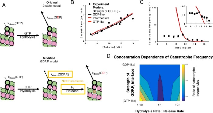
FIGURE 2: — Three-state model that contains a GDP.P_i intermediate. (A) Cartoons illustrating the differences between models without (top) and with (bottom) a GDP.P_i intermediate. The GDP.P_i intermediate requires two additional parameters: a rate constant for P_i release and another for the strength of the longitudinal interaction when GDP.P_i is at the interface. Vertical white arrows indicate trans-acting nucleotides. (B) Comparison between measured (black circles) and predicted (lines; red, black correspond to GDP.P_i interfaces having the same strength as GTP and GDP interfaces, respectively; brown corresponds to GDP.P_i interfaces having intermediate strength) growth rates. All three scenarios can recapitulate observed growth rates. In this plot the ratio between the hydrolysis rate and the phosphate release rates has been set to 1:1. (C) Predicted catastrophe frequency as a function of concentration for different values for the strength of the GDP.P_i longitudinal interface. Varying the strength of the GDP-P_i interface has a limited effect on the concentration dependence of the catastrophe frequency. The ratio between the hydrolysis rate and the phosphate release rates has been set to 1:1. The y-axis is linear in the larger plot. The smaller inset graph displays the same data, but the y-axis is on log scale. (D) Contour plot of the predicted concentration dependence of catastrophe. The concentration dependence is defined as the ratio of catastrophe frequencies at 9.5 and 13.5 µM. The concentration dependence of the catastrophe frequency is lowest when the ratio between hydrolysis and release is 1:1 and the longitudinal interface with GDP-P_i is as strong as the interface with GTP.