FIGURE 5:

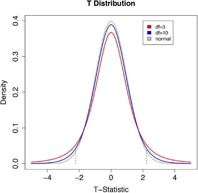
Comparison of two t distributions with degrees of freedom of 3 (sample size 4) and 10 (sample size 11) with a normal distribution with a mean value of 0 and SD = 1. The vertical dashed lines are 2.5th and 97.5th quantiles of the corresponding (same color) t distribution. The area below the left dashed line and above the right dashed line totals 5% of the total area under the curve. The t distribution is the theoretical probability of obtaining a given t statistic with many random samples from a population where the null hypothesis is true. The shape of the distribution depends on the sample size. The distribution is symmetric, centered on 0. The tails are thicker than a standard normal distribution, reflecting the higher chance of values away from the mean when both the mean and the variance are being estimated from a sample. The t distribution is a probability density function so the total area under the curve is equal to 1. The area under the curve between two x-axis (t statistic) values can be calculated using integration. With large sample sizes the accuracy of estimates of the true variance in an experiment increase and the t distribution converges on a standard normal distribution. To determine the probability of the observed statistic if the null hypothesis were true, one compares the t statistic from an experiment with the theoretical t distribution. For a one-sided test in the greater-than direction, the area above the observed t statistic is the p value. The 97.5th quantile has p = 0.025. For a one-sided test in the less-than direction, the area below the observed t statistic is the p value. The 2.5th quantile has p = 0.025 in this case. For a two-sided test, the p value is the sum of the area beyond the observed statistic and the area beyond the negative of the observed statistic. If this probability value (p value) is low, the data are not likely under the null hypothesis.