Figure 4.

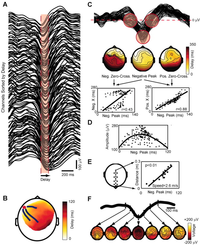
Each cycle of the slow oscillation propagates as a traveling wave. A shows the signals recorded from the channels affected by a single slow oscillation cycle ranked from top to bottom according to the delay of the negative peak. Note that the slow oscillation is not precisely synchronous in all channels and that a continuous distribution of time lags can be measured. The width of the red area represents the maximum delay (120 msec) from the negative peak at the top trace to the negative peak at the bottom trace. B depicts the spatial distribution of the delays on a delay map. A red asterisk marks the location of the channel with delay = 0 (the origin). The blue lines starting around the origin represent the streamlines calculated on the vector field of delays. The slow oscillation originates locally and propagates orderly to the rest of the scalp as a traveling wave. In C the same signals of A are superimposed; the red circles highlight the negative zero crossings, the negative peaks, and the positive zero crossings on the slow oscillation waveforms recorded from all electrodes. The maps below show the topographic distribution of the delays of these three reference points. The dots represent the channels affected by the slow oscillation, and the lines are iso-delay contours. Note that the spatial organization of the delays of the negative peak differs from that of the preceding negative zero crossings but is similar to that of the ensuing positive zero crossings. This observation is confirmed by the linear regressions performed between the delays of the negative peak (Neg. Peak) and those of the negative (Neg. X) and positive (Pos. X) zero crossings. In D, the peak-to-peak amplitude of the positive wave is plotted against the delay of the preceding negative peak. A parabolic function fits the points, indicating that the wave starts small and then waxes and wanes. E, The speed of wave propagation is measured from a row of electrodes placed on the anteroposterior axis (left). The slope of the linear correlation between the distance on the scalp and the measured delay gives the speed (right). F shows sequential voltage (average-reference) scalp maps calculated during different phases of the same cycle analyzed in the previous panels. The time of each map is indicated on the average of the slow oscillation signals recorded from all channels.