Figure 3.

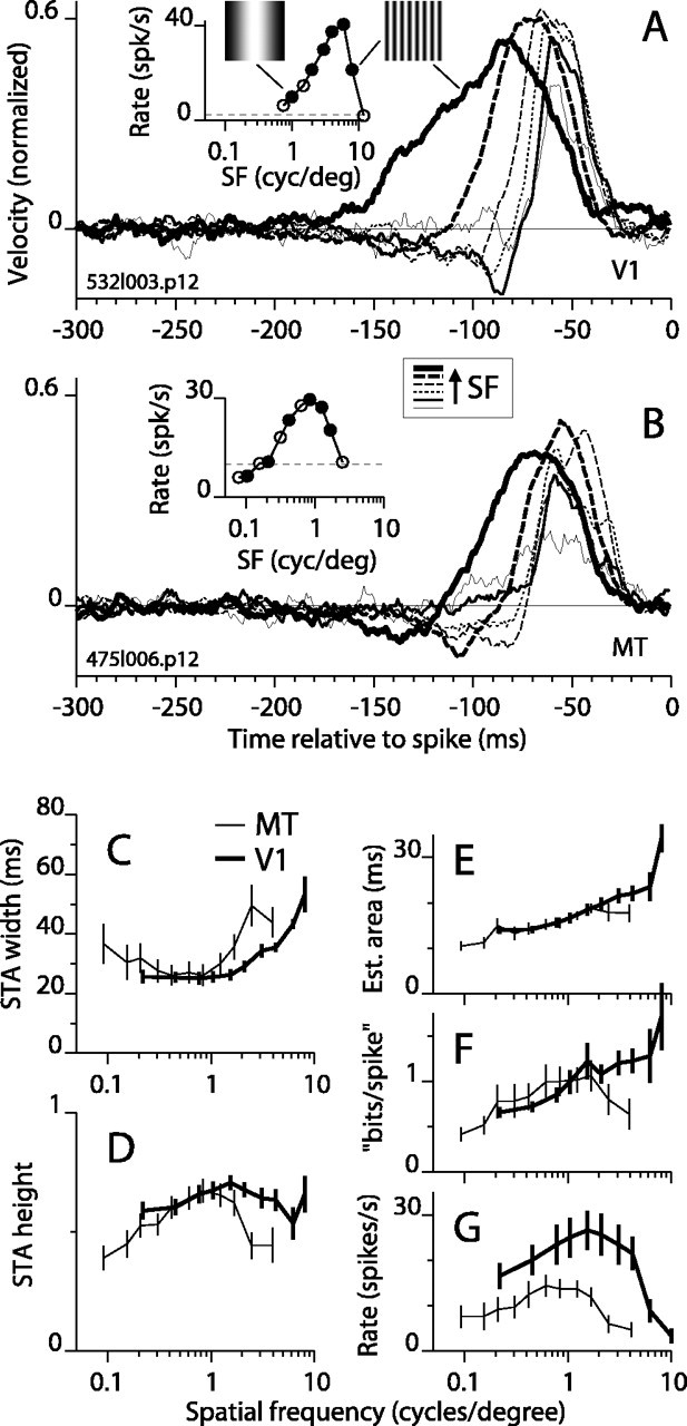
STAs as a function of grating SF. The format is the same as in Figure 2, except that SF is changing. A, STAs and firing rate for an example V1 cell. The icons in the spike rate inset show the visual stimuli drawn to scale for the lowest and highest (left and right, respectively) SFs that had STA peaks above the noise. High SF consistently yielded broad STAs (thickest line). The legend box between A and B shows the sequence of line styles from low to high SF. The optimal SF for drifting gratings (3 cycles/degree) corresponds to the short-dashed line. B, STAs and firing rate for an example MT cell. The optimal SF for drifting gratings corresponds to the thin long-dashed line. C-G, Same format as Figure 2, except the horizontal axis is SF. The actual SF values tested for each cell were typically not exactly those indicated by the points plotted here. The x coordinates used here are the average SF values for all points that fell in a cluster. The error bars show SEM.