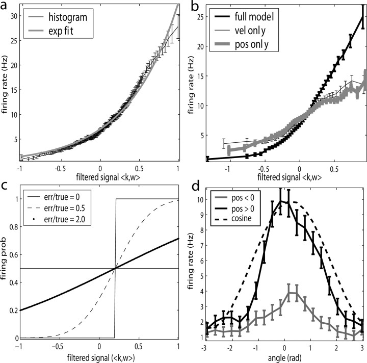
Figure 6.

Illustration and implications of the nonlinearity of MI cells. a, Example encoding function f (mean ± SE), with corresponding exponential fit. b, Observed encoding function f for filter set to extract optimal , position, or velocity along preferred direction. Tuning becomes sharper (more nonlinear) and observed dynamic range increases as chosen filter becomes closer to optimal . c, Illustration on simulated data of linearization effect on sharpness of nonlinearity. Model cell is perfectly binary, firing with probability one or zero depending on whether is larger or smaller than a threshold value. As the ratio of to becomes larger (i.e., as we project onto an axis that is farther away from the true ), the observed nonlinearity becomes shallower and smoother, becoming perfectly flat in the limit as becomes large. d, Dependence of velocity direction tuning curves (expected firing rate as a function of velocity angle) on hand position. Gray curve was computed using only velocities that were observed when hand position was to the left of midline; black curve used only rightward positions. Cosine curve (dashed) shown for comparison; observed tuning is significantly sharper than cosine (one-sided t test).