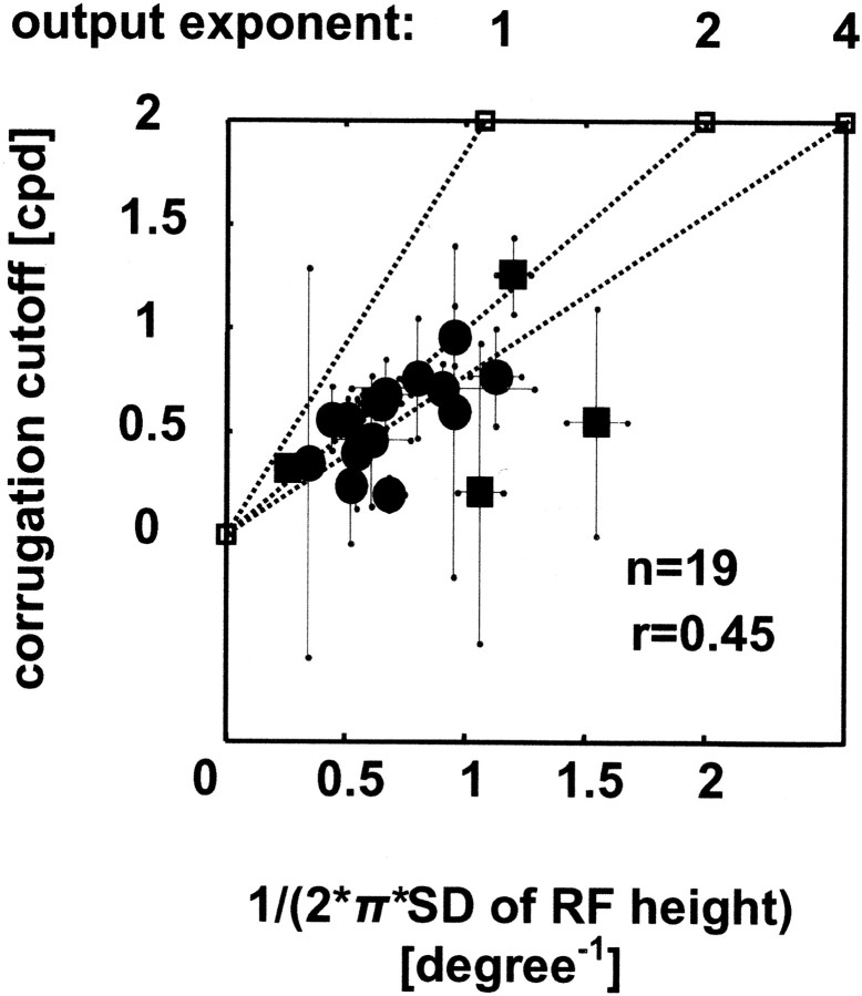
Figure 7.

The relationship between RF size (the SD of a Gaussian fit to responses like those in Fig. 6; SDrf) and high-frequency cutoff for depth corrugations (the SD of a lowpass Gaussian fit to data like those shown in Fig. 2E; SDsf). Because an inverse relationship is expected, 1/(2π^*SDrf) is plotted on the abscissa (i.e., the SD of the same Gaussian in the frequency domain). There is a significant correlation (r = 0.45; p < 0.05; n = 19). Circles and squares depict cells, for which the RF was measured monocularly in the dominant eye (n = 14) and binocularly (n = 5), respectively; the error bars correspond to SEs (by resampling). This relationship was also examined with the model (dotted lines). The model responses are shown for three different output exponents (1, 2, and 4). Note that no neuron lies significantly above the line predicted by the model with an output exponent of 2 (i.e., a half-squaring output nonlinearity). This line also represents the identity line. The output exponent of 1 refers simply to half-wave rectification, a sufficient nonlinearity to generate disparity selectivity.