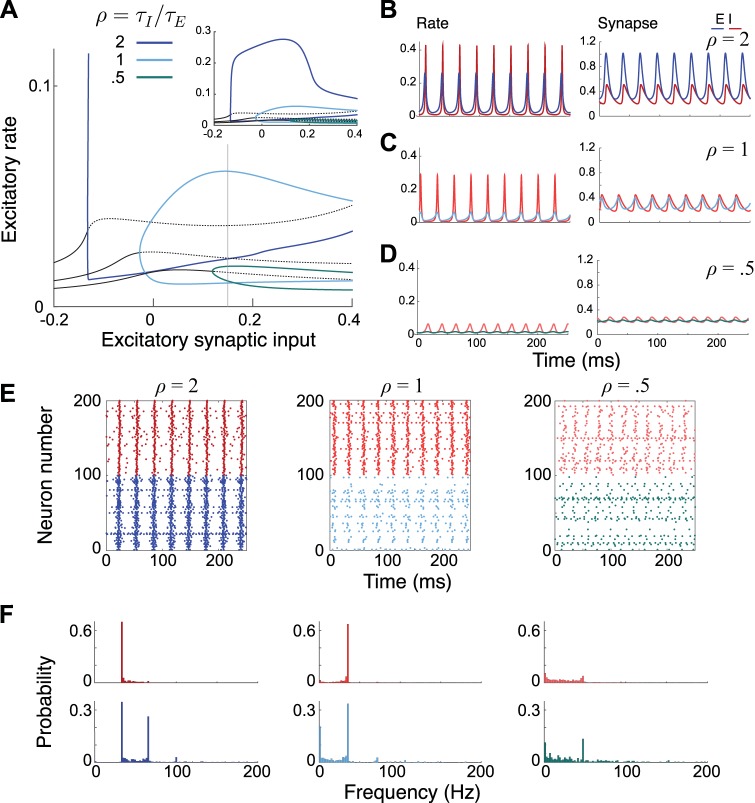
Fig. 3.

Behavior of the 2-population quadratic integrate-and-fire (QIF) model for 3 values of the ratio of the integration time constants, ρ = τ_I/τ_E. A: bifurcation diagram of the system described by Eqs. 8–10, showing the firing rate of the excitatory population as a function of the drive to the excitatory synapses $s_{\text{0}}^{\text{E}}$. Solid (dashed) black line represents the stable (unstable) steady state. Curves illustrate the minimum and maximum amplitude of the oscillations for various values of ρ. As in Fig. 2, the amplitude increase becomes more abrupt as ρ is increased. Inset: zoomed-out version of the entire bifurcation profile showing peak amplitude values. B–D: example time courses of the firing rate and synapses for the mean-field model, taken for $s_0^{\text{E}}$ = 0.15 (gray vertical line in A). E: raster plots of the individual neuron firing rates for a network of spiking QIF neurons. The raster plots show a random sample of 10% of the neurons in the network. The parameters are chosen to match those in A–D. F: distribution of firing rates of individual neurons in corresponding simulations. Neurons fractionally participate in oscillations with smaller ρ values, but the overall population frequency remains relatively constant. The integration time constants are given as τ_E = 8 ms and τ_I = 4 ms (ρ = 0.5), τ_E = τ_I = 6 ms (ρ = 1), and τ_E = 4 ms and τ_I = 8 ms (ρ = 2).