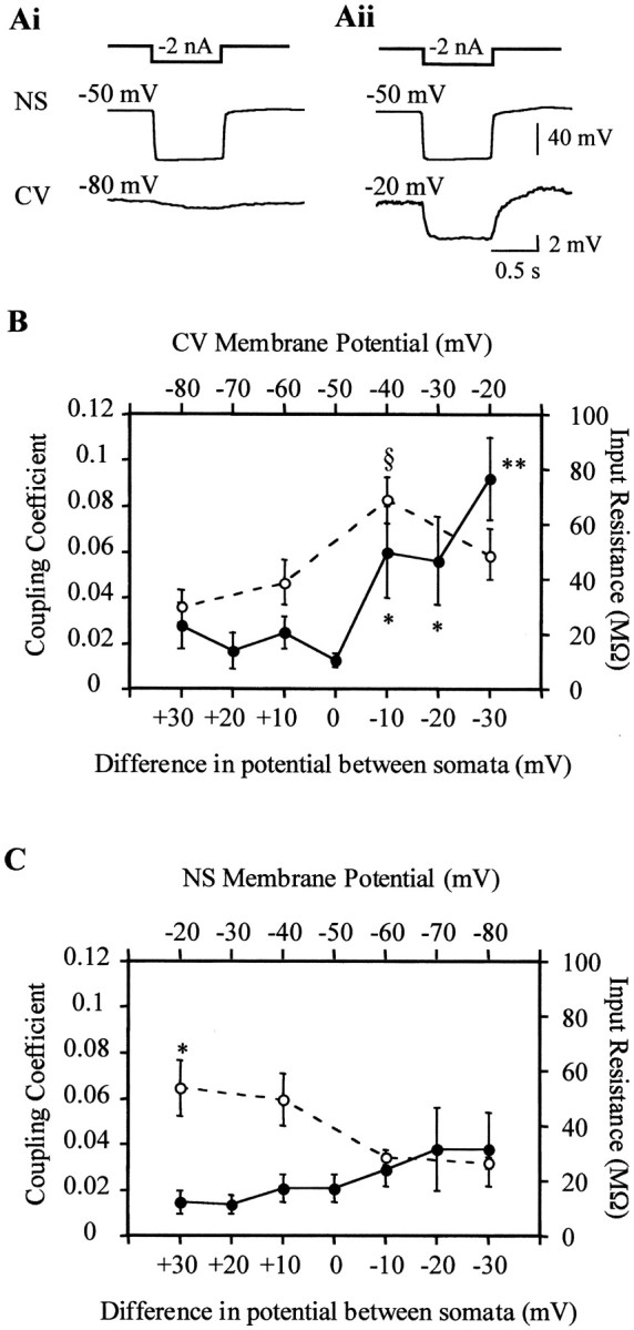
Fig. 4.

Coupling between NS neuron and CV motoneuron as a function of the transjunctional potential. A, Representative recordings showing the responses of an NS neuron and a CV motoneuron to a hyperpolarizing square pulse (represented by thesquare step line on top) injected in the NS neuron. The membrane potential of the NS neuron was set at −50 mV, whereas the membrane potential of the CV motoneuron was set at −80 mV (Ai) or −20 mV (Aii). B, The graph shows the coupling coefficient between CV and NS neurons (●) and the input resistance of the CV motoneurons (○) as a function of the membrane potential of the CV motoneuron (top axis) and of the difference in membrane potential between the NS neurons and the CV motoneurons (bottom axis), measured at the somata (Vm_NS −Vm_CV).^§ p < 0.01 (compared with each one of the other data points of the same curve); *p < 0.01 and **p < 0.001 (compared with the value obtained at no potential difference between somata). C, The graph shows the coupling coefficient between the CV motoneurons and the NS neurons (●) and the input resistance of the NS neurons (○) as a function of the membrane potential of the NS neuron (top axis) and of the difference in membrane potential between the CV motoneurons and the NS neurons (bottom axis), measured at the somata (Vm_NS −Vm_CV). *p < 0.01 (compared with the value obtained at a membrane potential of −80 mV). The coupling coefficient was calculated as the amplitude of the response displayed by the motoneuron (postsynaptic) over that displayed by the NS neuron (presynaptic). The symbols and error bars indicate mean and SEM, respectively (n= 15, for each case). Statistical analysis used two-factor ANOVA with repeated measures.