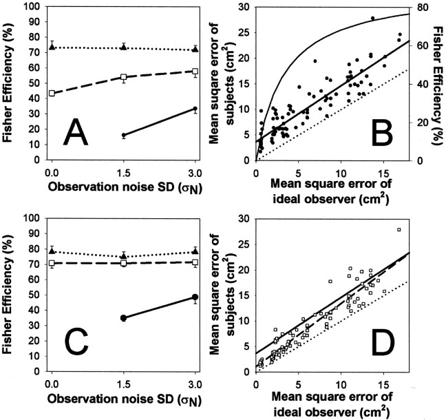
Fig. 4.
A, Subjects were very efficient (maximum 73%) at adapting to a random walk (with SD ςW). Data are plotted as Fisher efficiencies (the ratio of the mean square error of the ideal observer to the mean square error of the subject) across all conditions (●: no drift ςW = 0 cm; □: medium ςW = 0.75 cm; ▴: high drift ςW = 1.5 cm; mean efficiency ±1 SE; n = 12). B, Subjects' run-by-run performance versus ideal performance. Subjects' mean square error is plotted against the corresponding mean square error of the ideal observer (●, n = 96: 4 subjects × 8 conditions × 3 repetitions); the bold line is the regression. Thedotted line shows the performance of the ideal observer (i.e., slope equals 1 and intercept zero). The curve is an estimate of subjects' efficiency against the mean square errors of the ideal observer (Eq. 18), plotted against the axis on the right.The level of mean square error expected if subjects failed to track the drift component for ςW = 0.75 or 1.5 would be 19.7 and 78.9 cm2, respectively, in the absence of observation noise (ςN = 0). The mean squared displacement caused only by observation noise (ςW = 0) would be 2.0 and 8.2 cm2, for ςN = 1.5 and 3 cm, respectively. C, Fisher efficiency scores for subjects' performance when direct vision of the hand was allowed. The graph is in the same format as in Figure 4A. D, Run-by-run performance versus the ideal, with data from sessions with direct vision of the hand (□, n = 96), the regression of this data is shown by the bold dashed line. For comparison, the regression line from Figure 4B is also shown (no-vision, solid bold line).

