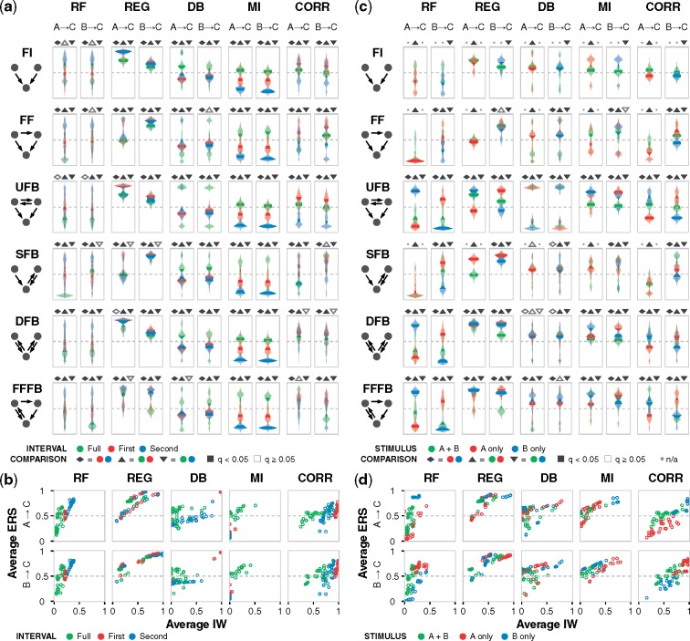
Fig. 3.

Performance depends on the sampled time interval and the stimulus target. (a) ERS distribution across the kinetic landscape for each algorithm, motif, and gate edge, with data for an OR gate and stimulus to nodes A and B. Violin plots for each landscape are color coded to reflect data sampled from the first half, second half, and full timecourse. Dashed lines indicate a confidence value of 0.5. Pairwise hypothesis testing for time intervals was performed using two-tailed Welch’s t-test, followed by multiple hypothesis correction using the Benjamini–Hochberg procedure for all tests within a given algorithm-edge group to obtain q values, as described in Materials and methods. Pairwise tests are indicated by the shapes above each subplot with statistically significant ($q<0.05$) outcomes filled-in. (b) Joint distribution of average IW and average ERS across the same landscape of motif-gate combinations and algorithm-edge groups. (c) ERS distribution for each algorithm, motif and gate edge, with data for an OR gate and data sampled from the full timecourse. Plots are color-coded based on node A, B, or both as the stimulus target(s). Absent violins are due to special cases that cannot be inferred (as algorithms do not interpret flat trajectories), and nonapplicable tests are denoted by a dot in place of a shape above subplots. (d) Joint distribution of average IW and average ERS. Additional simulation conditions and plots are in the Supplementary Material and online data browser