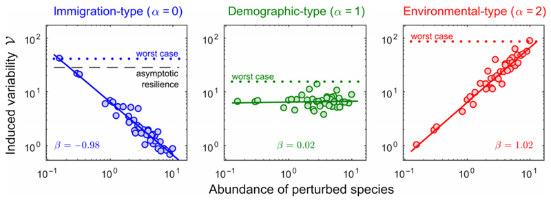
Figure 4.

Variability–abundance pattern in a complex community. We consider a community of S = 40 species, and look at the variability induced by perturbing a single species, whose abundance is reported on the x-axis. Left: When caused by immigration-type perturbations (α = 0), variability is inversely proportional to the abundance of the perturbed species (notice the log scales on both axis). The worst case is achieved by perturbing the rarest species, and is determined by asymptotic resilience (more precisely, it is close to 1=2ℛ_∞). Middle: For demographic-type perturbations (α = 1), variability is independent of the abundance of the perturbed species. The worst case is not necessarily achieved by focusing the perturbation on one particular species. Right: For environmental-type perturbations (α = 2), variability is directly proportional to the abundance of the perturbed species. The worst case is attained by perturbing the most abundant. The value β reported in each panel corresponds to the exponent of the fitted relationship $V_i\alpha N_i^{\beta }$ for each perturbation type α.