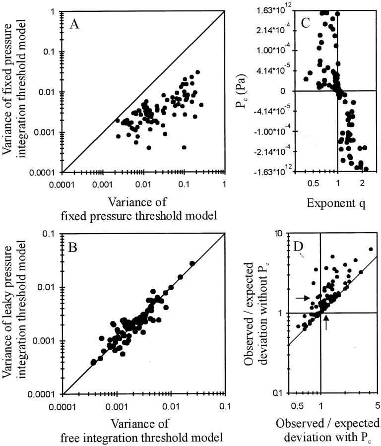
Fig. 7.
A, Scatterplot of the variance obtained with a fixed pressure integration threshold model versus that obtained with a fixed pressure threshold model. Both models have two free parameters, namely Lmin (in milliseconds) and threshold (in Pascal times millisecond and in Pascal, respectively). Solid line is the diagonal. Note that for all 89 AN fibers, the pressure integration threshold model provides a much better fit. B, Scatterplot of the variance obtained with a pressure integration threshold model with leakage/additional inflow versus the variance obtained with a free integration threshold model. Both have three free parameters and describe the data equally well. C, Scatterplot of pressure gain or loss (in Pascal), obtained from the fits with a pressure integration threshold model with leakage/additional inflow, versus the exponentq, obtained from fits with a free integration threshold model. Note that values of q greater (smaller) than 1 are associated with negative (positive) values ofPc, i.e., with pressure loss (pressure gain). Also note that the data are plotted along a nonlinearly transformed ordinate, where y = arctan(104 × x). This transformation offers high resolution near zero, where most values are located, and lower resolution of the fewer extreme values. A logarithmic axis is not useful, because Pccan be negative, and a linear axis does not allow the systematic trends around zero to be seen when all data are plotted. D, Scatterplot of the ratios between observed and expected deviations obtained with the fixed pressure integration threshold model (ordinate) against those ratios obtained with the pressure integration model with leakage or additional inflow (abscissa). For calculation of those deviations see Results. Arrows represent the geometrical means of the two distributions, and the oblique linerepresents the diagonal.

