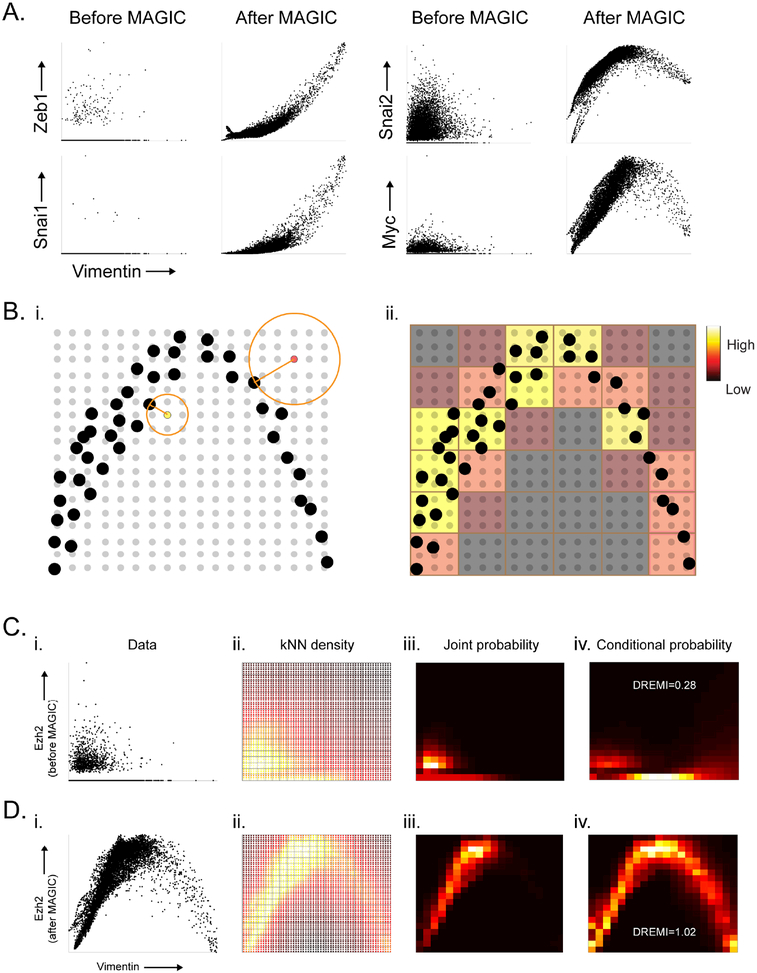
Fig. 5: Gene-Gene Relationships and kNN-DREMI.
A) 2D scatterplots before and after MAGIC. B) Illustrates the computation of kNN-based density estimation on an 18 × 18 grid, shown as gray points with data points shown in black. Each grid point (yellow, and red grid points are examples) is given density inversely proportional to the volume of a circle with radius r equal to the distance to its nearest data neighbor (black point). After density estimation on the grid-points, the grid is coarse grained into a 6×6 discrete density estimate (red and yellow squares show coarse grained partitions) by accumulation of all densities within each square bin. C) The steps for computing kNN-DREMI are shown for EZH2 (Y-axis) and VIM (X-axis) before MAGIC, with (i) a scatter plot, (ii) kNN-based density estimation on a fine grid (60×60), (iii) coarse-grained joint probability estimate on probability to obtain conditional probability density, resulting in 20 × 20 partition, and (iv) normalization of joint kNN-DREMI = 0.28. D) Same steps as (C) shown after MAGIC resulting in a kNN-DREMI = 1.02. See also Figure S5.

