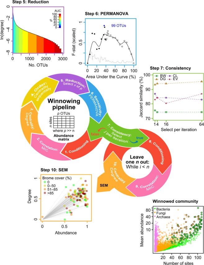
Fig. 1.

Conceptual diagram of the general winnowing and network prediction algorithms for microbial taxa with example results using degree centrality. Abundance data were conditioned using Laplace (add-1) smoothed [65] to reduce the undue influence of absent or rare species on subsequent network analyses (step 1). Correlation matrices were generated using maximal information coefficient (MIC) [50] (step 2). Centrality metrics drawn from graph theory highlight different aspects of changing microbial populations (step 3) [66] (see Supporting Information for results of the other centrality measures). Winnowed microbial communities were ordered by decreasing centrality (step 4) and a certain number selected (step 5) based on area under the curve (AUC) sensitivity analysis of the metric of interest. The selected operational taxonomic units (OTUs) were evaluated by treatment effect (i.e., brome-invaded versus natural grasslands; step 6) by testing the homogeneity of multivariate dispersions within groups using permutational analysis of variance (PERMANOVA) [52] at 5% AUC intervals. The F-statistic was scaled from 0 to 1 and spline-smoothed (solid line) to facilitate comparisons among the datasets. The dashed line indicates standard deviation calculated within a 5% moving window. Closed circles indicate retained taxa. Points were plotted at 1% intervals around each cut-off point. The number of sequentially ordered OTUs were selected to maximize the F-statistic and minimize the standard deviation (e.g., 99 OTUs in blue text). To test the consistency of the selection procedure, we ran a sensitivity analysis to evaluate the effect of parameter selection on the winnowing process conditioning for each centrality measure (select j OTUs per iteration; step 7). BW betweenness, CL closeness, DG degree, EV eigenvector. To generate the data used for the structural equation modeling (SEM), we iterated the winnowing pipeline in a leave-one-out procedure to quantify the contribution of each sample plot to abundance and centrality for each OTU (n = number of samples; steps 8–9). We used the sum of all OTU abundance-centrality distances to origin (step 10) as an endogenous variable in our SEM. Winnowed OTUs are represented by enlarged points with black outlines in the abundance versus occupancy plot