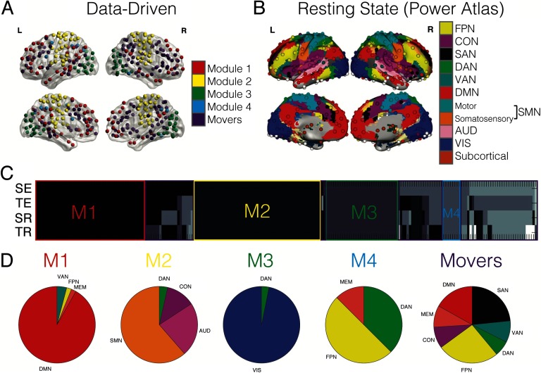
Figure 2. .
Data-driven community detection compared with RSNs. (A) The anatomical distribution of nodes used in the analyses is shown on the transparent brains (left and right, lateral and medial views). The color of the node indicates to which data-driven module each node belongs. (B) The anatomical distribution of nodes extracted in Power et al. (2011) with each resting-state network (RSN) indicated in the different colors (Figure from Cole et al., 2013). FPN = fronto-parietal; CON = cingulo-operculo; SAN = salience; DAN = dorsal attention; VAN = ventral attention; DMN = default mode; SMN = sensorimotor; AUD = auditory; VIS = visual. (C) The gray-scale matrix (4 conditions × 223 nodes) indicates the module identity for each node for each group-level network. SE = spatial encoding; TE = temporal encoding; SR = spatial retrieval; TR = temporal retrieval. Nodes belonging to the same module are the same color, resulting in four stable data-driven modules outlined in red, yellow, green, and blue. M1 = Module 1; M2 = Module 2; M3 = Module 3; M4 = Module 4. Any node boxed in purple is considered a flexible “mover” node, not belonging to a stable module. (D) Each pie chart shows the proportion of nodes from the RNSs that now belong to each data-driven module.

