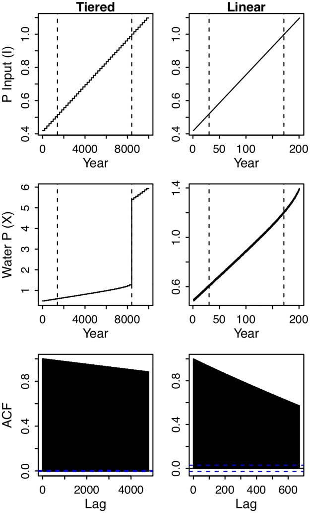
Fig 2. Time series of simulated lake phosphorus.

Simulations included 24 observations per year for the entire period of study. The first row shows time series of phosphorus input (I), the second row water phosphorus (X), and the third row the autocorrelation function. The left column of panels contains results from a simulation in which I was increased in a stepwise fashion; the model was initiated at equilibrium at the start of each tier of P input, each of which lasted 200 years. The maximum number of lags in the bottom-left panel is equal to the number of observations in 1 tier of P input (200*24). The right column of panels contain results from a simulation in which P input is increased smoothly and linearly over time; each time step has slightly higher I than the previous. The number of lags in the bottom-right panel are equal to the number of observations in 28 years. The vertical dashed lines indicate the times at which alternate equilibria emerge (a stable node and a saddle point), and when the original equilibrium (a stable node) is annihilated as it collides with a saddle point (see Fig 1). Both simulations are stochastic, but the simulation on the right includes an additional sinusoidal process. The simulation with smooth and linear increases in I (right) does not show an abrupt increase in X because the system is lagging behind its equilibrium value, which changes with I.