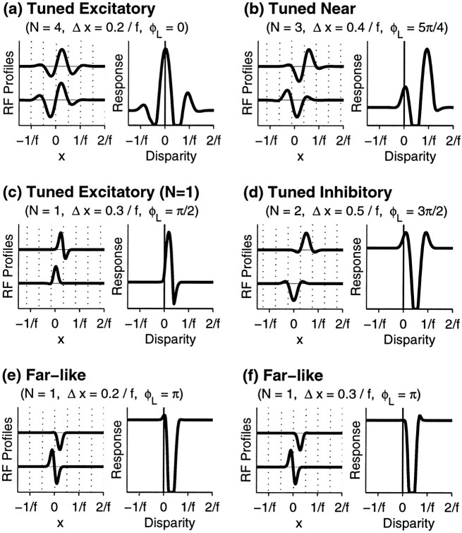
Fig. 5.
Examples of tuning curves for model binocular simple cells obeying the subregion correspondence hypothesis. For each cell, the number of subregions, N, is set equal in the left and right eyes. From this, we calculate ςRi = ςLi =N/(9.79fi). Note that this definition of N refers to the number of complete subregions (intervals between zero crossings, shown by dotted lines) that can fit within the RF, such that the RFs in c, e, andf are classified as N = 1. Parameters are given above each cell. a, Cell with four subregions and a small position shift gives a “tuned excitatory” response curve with a large peak at zero disparity and smaller side peaks atD = ±1/fi. b, Larger position shift gives a “tuned near” response: the main peak is now at D = +1/fi, whereas a smaller peak remains at D = 0. c, “Tuned excitatory” type cell with N = 1, which gives a response maximum shifted away from zero. d, “Tuned inhibitory” response curve for which inhibition is the most prominent feature. e, “Far-like” response curve with prominent suppression for positive disparities. f, Different type of “far-like” response curve.

