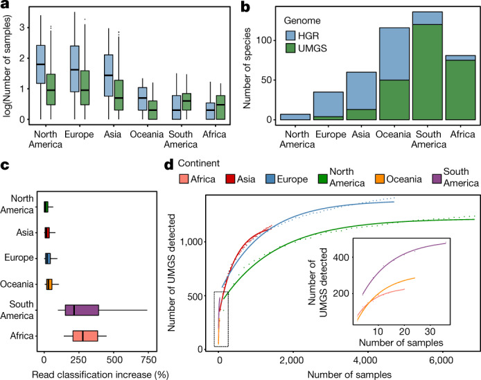
Fig. 4. Geographical distribution of the samples and uncultured species.

a, Distribution of the number of samples (log-transformed) that each HGR or UMGS present in at least one sample was found at a relative abundance above 0.01%. HGR genomes: n = 31 (Africa), n = 340 (Asia), n = 351 (Europe), n = 362 (North America), n = 86 (South America) and n = 129 (Oceania). UMGS genomes: n = 230 (Africa), n = 1,157 (Asia), n = 1,410 (Europe), n = 1,238 (North America), n = 482 (South America) and n = 287 (Oceania). b, Number of species found (abundance > 0.01%) in more than 20% of the samples from each geographical region. c, Percentage increase of the proportion of reads, partitioned by sample geographical location (Africa, n = 21; Asia, n = 1,447; Europe, n = 4,716; North America, n = 6,869; South America, n = 36; Oceania, n = 24), that were assigned to the HR, RefSeq and UMGS, in relation to HR and RefSeq alone. d, Accumulation curve depicting the number of UMGS detected as a function of the number of metagenomic samples per continent. Data points represent the average of ten bootstrap replicates. The curve of best fit generated from an asymptotic regression is represented for each geographical region. In a and c, box lengths represent the IQR of the data, and the whiskers the lowest and highest values within 1.5 times the IQR from the first and third quartiles, respectively.
