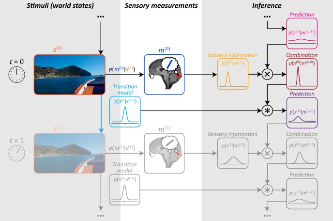
Figure 4.

Ideal observer in the natural environment. Illustration represents a single iteration in a continuous perceptual inference cycle. Left column represents the degree to which the environment remains stable over time, described by the transition model (light blue). For instance, edges in the environment (e.g., the one marked in orange) typically do not change much from one moment to the next. The ideal observer uses knowledge of these transition probabilities to infer the stimulus from its noisy sensory inputs. Specifically, at time t = 0, the observer takes a sensory measurement m⁽⁰⁾ of the stimulus s⁽⁰⁾ (an oriented edge). The measurement carries information about the stimulus, which is expressed by the probability distribution p(s⁽⁰⁾|m⁽⁰⁾) (yellow). This distribution is subsequently combined with a prediction (pink), which is based on previous sensory observations combined with knowledge of the environment's temporal statistics. The prediction is expressed by a probability distribution p(s⁽⁰⁾|m^(t₀:−1)), where t₀ denotes the starting point of the inference process that is arbitrarily long ago. The prediction is integrated with incoming sensory information to arrive at a combined distribution p(s⁽⁰⁾|m^(t₀:0)) (red), which reflects all sources of knowledge available to the observer at t = 0. Finally, the observer uses this perceptual knowledge available at time 0 to generate a new prediction p(s⁽¹⁾|m^(t₀:0)) (purple) about the next stimulus at time t = 1, and the cycle continues.