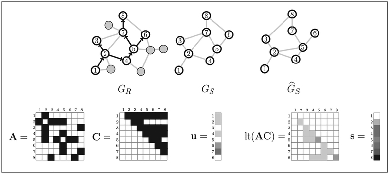
Figure 2.

Examples of matrices used to calculate the recruitment time series likelihood. At top left is the recruitment graph G_R overlaid on the population graph G, with recruited vertices numbered and other vertices and edges in gray. The true recruitment-induced subgraph G_S is not directly observed. We estimate G_S by ${\widehat{G}}_S$ and let A be the adjacency matrix of ${\widehat{G}}_S$. The coupon matrix C and the number of pendant edges attached to each recruited vertex is u. Pendant edges connect recruited vertices to unknown/unsampled vertices. The i, jth element of lt(AC) is the number of recruiters connected to i just before the jth recruitment event.