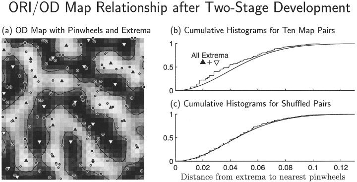
Fig. 13.

Data from the end of a two-stage simulation as in Figure 10c,d, but with a longer first stage: t₁ = 66. a, The gray scale image shows the OD map after smoothing with the Gaussian filter exp (−x²), with x measured in cortical grid intervals. Circles mark locations of singularities in the ORI map. Each upward- ordownward-pointing triangle marks a local maximum (maximum of right-eye preference) or minimum (maximum of left-eye preference) of OD, m(x⃗), in the smoothed OD map. b, Cumulative histogram (rough curve) of the distances, as a fraction of map width, connecting each of the OD maxima and minima in the smoothed map to its nearest ORI singularity, for the map in a and for nine other two-stage simulations with identical parameters but different seeds for the random-number generator. Thesmooth curve shows the distribution expected if local extrema and singularities were each independently and randomly located with a uniform probability density (spatially Poisson; Chandrasekhar, 1954); this curve is proportional to p(r) = 1 − exp (−λπr²), where λ = 116.0 is the average number of singularities per ORI map. The observed distribution contains more small distances (mean, 0.0422) than the expected distribution (mean 1/2 $\sqrt{\lambda }$ = 0.0464). The two distributions are significantly different [p_KS < 8.17 × 10⁻⁸, where p_KS is the p value from Kolmolgorov–Smirnov (KS) test]. This effect weakens as the length of the first stage, t₁, is decreased and is very weak or absent for one-stage development. c, The “shuffled” cumulative histogram (rough curve) was obtained by matching pairs of ORI and OD maps from simulations using different seeds. This curve lies much nearer to and has the same mean value (0.0464) as the random distribution. Even though the histograms in b and c are clearly different, because there are many more data points underlying the shuffled histogram in c than the single-run histogram in b, the difference between shuffled and random distributions has only a slightly weaker p value (p_KS < 1.64 × 10⁻⁵) for c than b.