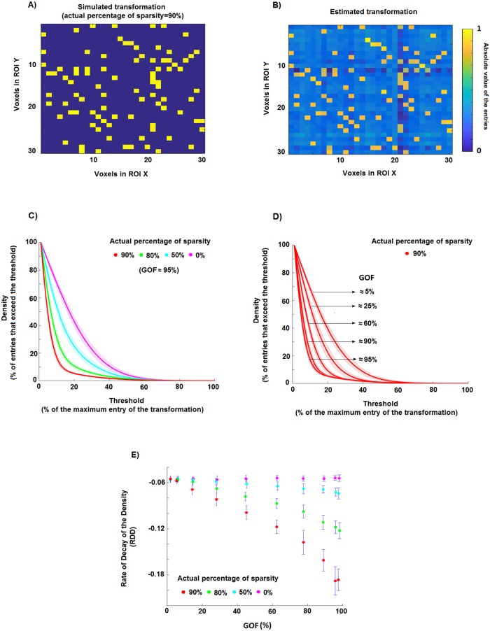
Fig 2. Estimation of the percentage of sparsity using a ridge regression method.

A) An example of a simple sparse simulated transformation: 90% of the entries are equal to 0, while the other 10% of the entries are equal to 1. B) Estimate of the transformation in A obtained by using the ridge regression method. The lighter background indicates that the estimated elements are different from zero even if in the original transformations they are exactly equal to zero. C) Density of the thresholded estimated transformations, i.e. the percentage of matrix entries that exceed the threshold, as a function of the threshold. In this toy example, we generated 30 realisations for four simulated percentages of sparsity (0%, 50%, 80% and 90%). D) Density of the thresholded estimated transformations associated with a degree of sparsity of 90% and different GOF values (i.e. different levels of noise in the model). E) Scatter plots of the rate of decay of the density curves (RDD) shown in panel C against goodness-of-fit GOF for the 30 simulation realisations of each of the four different cases. It is evident that simulated transformations of e.g. 90% sparsity are associated with a certain range of RDD and GOF values (red dots) which, at least for sufficiently large values of GOF, are different from those related to transformations with 80% of sparsity (green dots).