The Heterogeneity problem: Approaches to identify psychiatric subtypes

Abstract

The imprecise nature of psychiatric nosology restricts progress towards characterizing/treating mental health disorders. One issue is the ‘heterogeneity problem’: different causal mechanisms may relate to the same disorder, and multiple outcomes of interest can occur within one individual. Our review tackles this ‘heterogeneity problem’, providing considerations/concepts/approaches for investigators examining human cognition and mental health. We highlight the difficulty of pure dimensional approaches due to ‘the curse of dimensionality’. Computationally, we consider supervised and unsupervised statistical approaches to identify putative subtypes within a population. However, we emphasize that subtype identification should be linked to a particular outcome or question. We conclude with novel hybrid approaches that can identify subtypes tied to outcomes, and may help advance precision diagnostic and treatment tools.

Mechanisms underlying mental health issues are mostly unknown

For over 100 years[1–3] psychiatrists, psychologists, and mental health providers have developed and refined psychiatric nosology via efforts that include a series of revisions of the World Health Organization’s International Classification of Disorders (ICD; see: Glossary) [4] and the American Psychiatric Association’s Diagnostic and Statistical Manual for Mental Disorders (DSM) [5] (see Box 1 and Box 2). Critically, the validity of this approach has relied on using phenotypic data to identify putative ‘clinical types’ [6] which are necessary, as of now, for clinical decision making. However, despite the competing practical interests that drive the official nosology, the need for more effective tools to discover pathophysiology has led some recently to a drive for alternatives [7–12]. The primary concerns with the DSM and ICD nosology for psychiatry are well known and comprise both over-and under specificity, that is: (a) heavy overlap among the “disorders,” and shared biological features, indicating a lack of clear natural boundaries for defining disorder presence or absence (many exist on a continuum), and (b) substantial heterogeneity within each condition[10,12,13]. This latter point, heterogeneity, includes the issue that different mechanisms may drive diagnosis for different subsets of individuals, here called “subtypes” (see Box 1). Therefore, biological measures may differ for one subtype, but not another. As a result, some biological markers may only be found within a subset of individuals for a given diagnosis [14,15]. While the problem is well known, the solution is unclear[16]. The present review therefore offers further thoughts on this ‘heterogeneity problem’ (see: Box 1) and provides considerations, concepts, and approaches for investigators examining typical and atypical cognition and mental health in human populations.

Box 1: Defining the heterogeneity problem.

In the current work we refer to The “Heterogeneity Problem” as a widely recognized and bi-faceted issue that some experts believe limits mental health and cognitive neuroscience research. Ultimately, an appropriate conceptual model that encompasses the natural heterogeneity of human outcomes is needed (see [104], as well as discussion in [105]). To that end, we must contend with two inescapable tenets. The first tenet refers to an understanding that any human mental health syndrome or outcome, from cognitive functions to clinical disorders, will not necessarily be ‘caused’ by a single mechanism; rather, because these conditions are multi-determined, they can be ‘caused’ by different combinations of inputs (also referred to as “equifinality”[106]). Importantly, such possibilities exist not only in clinical populations, but typical populations as well (e.g., study of normal trait variation). While this recognition is not new [63,64,104], methods to handle and in particular, to mathematically model, this problem continue to be refined and developed as we discuss in this article.

The second tenet refers to an understanding that outcomes related to single individual are vast and depend on the domain of interest (e.g., mood, education, health), which change the relevant heterogeneity parameters for that individual. In other words, when we try to identify a ‘mechanism,’ or rather pattern of features, related to a specific disorder or symptom, the ‘valid’ patterns depend on the specifics of the questions being asked. For example, the brain measures that differentiate a group of individuals with and without ADHD might be different than those brain measures that predict individuals who will have persistent ADHD symptoms over time, relative to regressive symptoms in later years (which would be distinct again from those measures that might differentiate individuals who will respond to cognitive therapy from those that will not). This particular issue, of course, pertains to any putative pathophysiological feature, not just brain imaging. In other words, when trying to understand and parse the variance amongst multiple features (brain, environment, demographics, etc.) in typical and atypical populations, many distinct sub-populations might emerge from such data. Each way of grouping them might be “valid” for a different purpose. Thus, no one ‘valid’ answer exists. A given solution depends on A) the features used to generate the model, B) the biases of the modeling strategy, and C) the goal or question at hand. As we argue in this review, supervised and unsupervised approaches to subtype populations have been informative and growing in the field with this regard; however, a weakness that we highlight is that most applications of these approaches do not identify subtypes tied to (C) the question of interest. As a result, such applications fall prey to this aspect of ‘the heterogeneity problem’ - identified subtypes that may be irrelevant to the question or outcome of interest. By tying subtype identification to the question of interest, hybrid approaches that combine with supervised and unsupervised characteristics may assist in modeling or capturing this aspect of the heterogeneity problem.

Box 2: Emergence of modern psychiatric nosology.

Taxonomies of mental disorder date from ancient times. In the West, they trace through Enlightenment and modern era developments in psychology of temperament and personality (for a review see [2,107]) and medicine (for reviews see [1,3,105,108]). As the cited reviews detail, the enterprise faces perennial epistemological and ontological issues [109,110]. Heuristically, one view presumes natural kinds in nature and seeks to map them to their hidden, process-based structure. The second camp, ascendant in the enlightenment, eschews etiology as speculative and instead emphasizes observable features that may cluster together. Cross cutting these views is the ontological question of whether nature holds true kinds, or whether the nosology is inevitably an arbitrary but useful convention with the “best” structure dependent on the purpose. In modern times, competing psychiatric classifications, drawing upon these competing philosophical approaches, were formalized in the 19^th and 20^th centuries and became standardized in response to the exigencies of world war II (DSM-II, 1952). The mid-20^th century re-discovery of the kappa statistic and its application in clinical psychology, and concomitant realization in psychiatry of the poor inter-clinician agreement on diagnoses in the 1960’s, provoked disillusionment with the etiological assumptions of DSM-II. An emphasis on descriptive nosology, albeit with a presumed biological theory, heavily influenced by the work of Robins & Guze [6], again took precedence and guided creation of nomothetic symptom lists for DSM-III (1980). DSM-IIIR (1987), DSM-IV (1994), and DSM-5 (2013) did not fundamentally change this approach (although an effort was made in DSM-IV and DSM-5 to acknowledge cross-cutting dimensions in psychopathology). It also failed and continues to fail to incorporate advances in the empirical description of psychopathology dating back over a half century [64,66,67] such that a unified approach is still lacking. Fundamentally, however, as has been noted for centuries, a purely descriptive nosology inevitably confounds multiple entities from an etiological perspective, while an etiological approach remains necessarily speculative in psychiatry at present. At present, despite some progress, concerns are salient regarding excessive reification of the DSM nosology and evidence that the nosology, whatever its practical advantages, does not reflect biological systems. All this has led to a desire for alternative proposals [63,111] at least for purposes of discovery pathophysiology, with some hope deriving from mathematical and empirical approaches [64,112] as this article testifies, although those approaches do not relieve us of philosophical choices and assumptions.

The heterogeneity problem challenges studies of mental health research

While the search for environmental influences on, behavioral, physiologic, and biologic markers of mental health conditions (and many complex cognitive behaviors) has been ongoing for centuries (see: Box 2), progress has been frustratingly slow. In the DSM era, the modal study often involves comparing a group of subjects with one of the disorders defined by core symptoms (e.g., via DSM criteria) to a group of control subjects without the disorder. Statistical group differences based on environmental influences, psychometrics, neuroimaging, or genomics are then used to inform models of the (putative) disorder’s pathophysiology or etiology. For example, increased functional connectivity between posterior cingulate cortex (PCC) and lateral orbitofrontal cortex (OFC) was recently suggested to be the mechanism for depression and its amelioration [17]. Indeed, “Undifferentiated brain states” observed from functional connectivity magnetic resonance imaging (fcMRI) has been suggested as an etiology for autism spectrum disorders (ASD) as well [18]. In attention deficit hyperactivity disorder (ADHD) it has been suggested that whole-brain immature functional connections may underlie the disorder[19]; others have proposed a cognitive and neural “footprint” of ADHD, where differential maturation of task control systems differentiate children with ADHD from typically developing children[20]. Similarly, polygenic risk scores [8,9,21–24] and large scale genomic studies [25]have been used in an effort to elucidate the etiology of various mental health disorders.

By design, such case-control studies are forced to implicitly assume that the given condition is a homogenous entity. However, this expectation of homogeneity makes two assumptions that are likely incorrect: 1) That a given disorder represents a single, mechanistically homogenous patient population, and; 2) That the typical population likewise represents a largely homogeneous and presumably more adaptive or optimal state[26].

Evidence suggests that major psychiatric conditions are heterogeneous

While a plurality of inputs to a given psychiatric presentation has been proposed recently in DSM-5[27] and for far longer in the literature [28], accumulating and recent evidence documents that this is, in fact, almost certainly the case for most psychiatric domains[29]. To give just some examples, heritability and genome wide association studies find profound heterogeneity in ASD[30–32]; common variants contribute to the heritability of the condition[30,31], while rare variants apparently contribute to symptom type and severity [30,32]. In short, the manifestation of ASD symptoms in a given individual may arise from fundamentally different mechanisms. Such heterogeneity is consistent with findings from predictive models of ASD using structural magnetic resonance imaging (sMRI) and functional magnetic resonance imaging (fMRI) data as well [33–37].

As another example, predictive models of future major depressive episodes or treatment outcomes in individuals show poor performance on independent datasets collected at different sites (e.g., Predicting response to depression treatment (PREDICT)[38], collaborative care management (CCM) [39], early medication change (EMC)[40], genome-based therapeutic drugs for depression (GENDEP) [41], or combining medications to enhance depression outcomes (COMED) [42]). However, using external data to reduce sample heterogeneity among individuals with a history of MDD may improve the generalizability of such predictive models. One study improved the prediction of depression treatment outcomes using externally acquired fMRI data. This was done first, by identifying computationally distinct MDD subgroups with different fMRI profiles, and then improving model performance by treating the subgroups as independent populations [38]. In this case, connectivity between the subcallosal cingulate cortex and left insula, dorsal midbrain, and left ventromedial prefrontal cortex dissociated reliably between two putative subtypes. One subtype showed high (i.e. positive) connectivity and were best treated by cognitive behavioral therapy but not medication, the other subtype showed low (i.e. negative) connectivity and were best treated by medication but not cognitive behavioral therapy. Similarly, genomic[43], behavioral[44], and fMRI [45] data may be promisingly used with newer computational methods to identify and/or help validate ADHD subgroups, although this work is still in its infancy[46]. Furthermore, such identified subtypes (e.g. as in [38], see also [47]) may not generalize to independent datasets across different sites[48], and therefore require additional independent validation (see Box: 3).

Box 3: On the interpretability and validity of predictive models.

Supervised, unsupervised, and hybrid modelling approaches comprise powerful methods to identify subtypes that may better characterize typical and atypical populations. Such models depend on approaches that estimate performance, called cross-validation (CV), and approaches that select the measures used to build the model, called feature selection (FS). In CV, participant datasets are partitioned evenly into folds. Per iteration, each fold is separated as a test dataset, and the remaining folds form the training dataset. By dividing participants into training and test datasets, testing is kept independent from the training process, which prevents overfitting. However, one must determine the number of folds to perform cross-validation. One commonly used approach, called LOOCV, is to make each subject its own fold. Although routine in neuroimaging[113], LOOCV poorly estimates model performance[114–116] compared to using 5 or 10 folds[114–116]. Even if modelling approaches adopt good cross-validation strategies, overfitting may still occur if improper FS strategies are implemented. FS involves selecting a subset of features to use in a given model, which helps overcome the curse of dimensionality. Optimal FS strategies determine the appropriate feature subset from the training data and not the testing data[117]. Models that use features selected from overlapping training and testing datasets often show inflated performance and fail to generalize to independent datasets[118]. Finally, inferences from models are limited by sample size. Small samples will generate greater variability in model performance, but models that perform well are more likely to be published[119–121]. Often, published predictive models of a given disorder usually decrease in performance as the reported sample size increases[33,35,122]. If good standards and practices are not adopted for CV and FS, models may perform poorly on new cases.

However, even if the best standards and practices are adopted, identified subtypes from models require independent validation. Independent datasets help verify models and improve performance when models do not perform well. Secondary measures help validate identified subtypes and refine inferences regarding clinical distinctions or biological relevance. These techniques can be combined to better validate putative subtypes. For example, assume that ASD subtypes were identified from a sample of imaging data using the FRF. To verify that such subtypes are linked to ASD affected behaviors, one could construct a predictive model of the subgroups from such behavioral data. One could then apply this behavioral predictive model to an independent set of ASD cases, to test the generalizability of the subtypes.

Evidence suggests that typical populations are heterogeneous

While heterogeneity within psychiatric syndromes is generally acknowledged, at least in theory, heterogeneity within the control group is rarely considered in the psychiatric literature (although it is well known in other fields such as personality and social psychology). Thus, the heterogeneity problem almost certainly applies to typical populations as well. When comparing typically developing individuals to individuals diagnosed with a given condition, researchers are often obliged to implicitly assume the Myth of Optimality[49] - the assumption that the typical population represents one homogenous and optimal state. However, typical samples vary widely in cognitive ability and intelligence[50]; emotional coping style [51,52]; genetic make-up;[53] and social niche[54–56], not to mention psychological adaptation or health. For example, individuals with similar overall IQ may cluster into different cognitive subgroups, where one such subgroup scores higher in verbal comprehension than another. However, both are associated with differences in temporal lobe morphology compared to a third group [50] and without evidence of maladaptation. In the case of working memory it is becoming clear that individuals can optimize this well studied cognitive function despite adopting different strategies, which are likely associated with different neural pathways [57]. Such variability in the typical population found in executive function measures may be critically important context for understanding mental health conditions, like ADHD [58]. In other words, these typical variations, may underlie or present distinct contexts for the presentation of a psychiatric condition—that is, the psychiatric conditions may be nested within typical heterogeneity [26,59].

Such implicit design assumptions related to typical and atypical populations may contribute to the frequently small effect sizes in psychopathology research. Clinically, these same assumptions may account for why treatment studies may show weak effects or have limited reproducibility. In short, assumptions of homogeneity within psychiatric conditions and among comparison groups have likely limited discovery with regard to identifying etiology, biological markers, and effective treatment options. There are several challenges which have made it difficult to overcome these assumptions in practice, even if they are understood to be incorrect in theory.

The ‘Curse of Dimensionality’ and the heterogeneity problem

Dating back many decades, one approach to overcome the heterogeneity problem in psychiatry has emphasized a dimensional logic to nosology[60–67], where extreme tails of a multi-dimensional continuous distribution (i.e. outliers) may indicate individuals that would benefit from treatment. Dimensions in this case would measure any combination of continuous or categorical variables that might include behavioral (i.e., performance on one or multiple tasks), biological (e.g. one or multiple genetic markers or brain features), environmental (i.e., one or more exposures), or other features. Unfortunately, while this approach might potentially reflect natural trait variation related to psychiatric nosology, it has major limitations in relation to actual clinical application. To detect outliers in such a scenario, one must first generate a representation of the population across the multi-dimensional space. While one can procure a sufficient sample size to measure a single dimension[68], it is a challenge to represent a population across multiple dimensions without considering subtypes. The reason relates to the “curse of dimensionality[69].”

To explain, if we were to measure the continuity of a dimension within the human population, say for example height (see: Figure 1a), one must decide to adopt some basic requirements for this distribution. Let us assume that the true distribution of height is Gaussian; the distribution is bell-shaped with a mean of 100 and a standard deviation of 5. To properly identify a population outlier in this simple case, an estimate of the distribution must first be generated. That estimate is based on your study sample. As the number of cases sampled in your study (i.e., from the distribution; illustrated in Figure 1a on the leftmost panels) increases from 10 to 300 (Figure 1a; top row), our estimate of the distribution better reflects the true distribution (blue arrows). Not surprisingly, the better that your sample reflects the true distribution, the better you are at identifying true population outliers. In this example, at 50 cases, more than 70 percent of true population outliers can be correctly detected (Figure 1b: left panel). However, if we want to identify outliers across two dimensions, let’s say height and weight, the intersection of the two dimensions generates a much larger search space than the 1-dimension example (Figure 1a; bottom row). Here, sampling 50 participants is insufficient (red arrow) to represent the true distribution (Figure 1a; “50 samples” bottom panel), and would be a poor sample to be able to accurately identify outliers. With that said, sampling 300 cases creates a better representation (blue arrow) of the population (Figure 1a; “300 samples” bottom panel). In this scenario, while correct outlier detection remains highly variable, true population outliers can still be detected better than 70 percent of the time on average (Figure 1b; middle panel). However, with three dimensions, let’s say height, weight, and education level, the search space grows exponentially. The true distribution cannot be modeled properly even with a large number of participants. Indeed, correct identification of population outliers is lower than the 2-dimension case even when 1000 individuals are sampled (Figure 1b; right panel).

Figure 1. Data simulations showing the ‘curse of dimensionality.’.

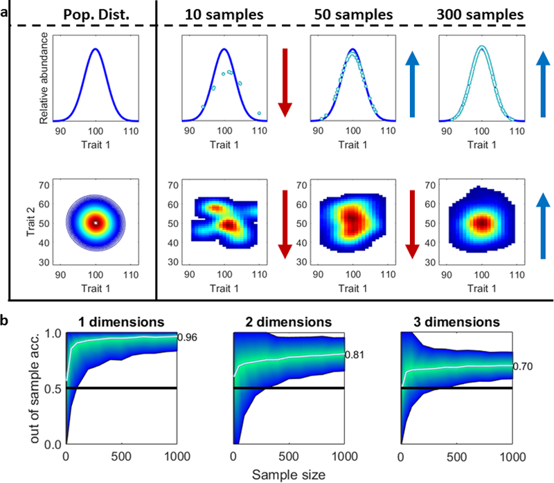
[69] Examining mental health disorders or cognitive behaviors considering only 1-continuous distribution using a purely dimensional framework (i.e., without considering subtypes) is challenging. (A). Data were simulated for correlated traits from Gaussian distributions (i.e., “Pop Dist.”). Trait 1 measure (x-axis) and frequency (y-axis) is plotted in the top row. The two dimensional density for traits 1 (x-axis) and 2 (y-axis) are plotted in the bottom row. The leftmost panels show the population distributions for the traits. From there we randomly sample “subjects” from the distribution. As shown, the number of “subjects” needed to approximate the distribution rises from 10 samples to 300 samples as the number of dimensions (i.e. traits) increases from one (top) to two (bottom). Good (blue arrows) and poor (red arrows) population fits are indicated. (B) Outlier detection was conducted [124] for one (left), two (middle), and three dimensions (right). Data were sampled from a multivariate normal distribution (means = 0, s.d = 1), to satisfy the method used. Thresholds for true outliers were determined from a large sample (N=10,000). To test outlier accuracy, smaller samples (N= 10 to N = 1000) were pseudo-randomly generated 1000 times and true outliers identified using the known threshold. Correctly identified outliers were calculated as the percentage of identified true outliers divided by the total true outliers. As shown, the accuracy of identifying true outliers decreases as the number of dimensions is examined. Code to reproduce these plots can be found at (http://github.com/dcan-labs).

When applying our example use-case and attempting to detect outliers accurately (Figure 1b), our performance decreases exponentially with increasing dimensionality. To become more accurate with increasing dimensional space requires exponentially more cases (i.e., subjects) to accurately detect outliers. By way of comparison, the Research Domain Criteria (RDOC) in its current iteration contains 22 categories measuring 44 dimensions [70]. The brain, of course, is likely to have even more signals or dimensions than this. Admittedly, other models of psychology make do with only a handful of dimensions [71], but the difficulty remains.

On the other hand, if one assumes that the population is comprised of multiple subtypes with different underlying distributions[69,72], then instead of detecting outliers one aims to distinguish boundaries between subtypes. In order to delineate such boundaries, one would need to define margins that separate the subtypes by measuring the overlapping space between them. Therefore, incorporating subtypes constrains the space that needs to be measured[73] - reducing the number of cases needed to identify generalizable boundaries. Here, relevant dimensions can help to identify and refine subgroups. Because subtypes may only be associated with a few relevant dimensions, it enables one to reduce the dimensionality, and the required sample size needed for delineation and analyses.

Several approaches can now identify subtypes in research

While the 20^th century saw heavy application of factor analysis to the issue of heterogeneity, more recent 21^st century developments in computational sciences and mathematics, have enabled the implementation of models that may be sufficiently complex to better address the aforementioned situation regarding subtypes. These approaches can be classically split into ‘Supervised’ and ‘Unsupervised’ methods.

Supervised approaches.

Supervised approaches (whether in statistics or in machine learning) make explicit assumptions about subtypes and then forces the data to fit these assumptions. In this case, if we know what dimensions may delineate subtypes we can develop a model to fit indicators of the given dimensions and predict subtypes. Such approaches are top-down and theoretically motivated[74]. One such approach extends from dynamic causal modelling (DCM), and is similar to popular methods such as latent class analysis or finite fixture models (noted below). In this approach, the number and shape of subtypes must be specified for each model. Other examples include mixture models, such as latent trajectory growth mixture models to identify ADHD trajectory subtypes [75] and latent class analysis to examine ASD subtypes[76–78]. These models have important strengths; in particular, they are helpful for confirming hypothesis driven nosology, analogous to confirmatory factor models. They have shown some promise in predicting diagnosis. The assumptions make it is easy to draw inferences from supervised models and test hypothesis regarding psychiatric nosology. Such approaches have been well-established outside of psychiatry[79].

On the other hand, supervised approaches make assumptions regarding the answer. Supervised models are biased towards the assumptions made, and therefore are limited by how much the assumptions are informed by prior knowledge. To take a real world example, if we were to try to identify the dialect for “carbonated beverage” across the United States, assuming two dialects (“soda” and “pop”), we would likely ignore the fact that most of the southeast says “coke” (see Key Figure, Figure 2a). An analogous clinical example is discussed below (see: Human population is profoundly heterogeneous across multiple dimensions).

Figure 2. Key Figure. U.S. populations maps reveal profound heterogeneity.

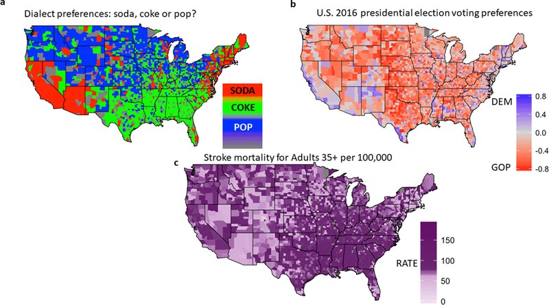
Several valid and important ways that a population might be subdivided are shown here. Each one of these subdivisions are useful for different types of questions and analogous to parsing clinical and cognitive heterogeneity. (A) Subtypes across the United States based on dialect preferences for ‘soda’, ‘pop’, or ‘coke’. Counties are colored by the most commonly used term. Language preferences were derived from Alan McConchie’s “pop vs. soda” survey (http://popvsoda.com/). Three subtypes were identified by the survey. East/West coast form one subtype that uses “soda”. Southeast people use “coke”, perhaps reflecting that Coca-Cola is headquartered in Atlanta. The northern/upper Midwest uses “pop”. (B) Subtypes across the United States based on the 2016 presidential election. Data were from Tony McGovern’s repository (https://github.com/tonmcg/County_Level_Election_Results_12–16). Difference between Democrat (blue) and Republican (red) voting percentages are plotted by county. Two subtypes can be seen from voting preferences. “Urban” counties centered around cities typically voted more Democrat. “Rural” counties typically voted more Republican. (C) Subtypes across the United States using data from the National Center for Health Statistics (https://www.cdc.gov/nchs/data_access/vitalstatsonline.htm). Stroke mortality rates for adults aged 35 years or older are plotted by county. One cluster can be seen in the eastern states, excluding the Northeast and tip of Florida, and another can be seen on the West coast. Code to reproduce these maps (http://github.com/dcan-labs) was written in R with the ggplot2[125] and maps[126] package. Color bar was resized and relabeled for visibility in this figure.

Unsupervised approaches.

Unsupervised approaches identify clusters from the structure or shape of the data itself. They may be thought of as “bottom up”. For example, hierarchical taxonomy of psychopathology (HiTOP) is a recently proposed a new taxonomy for psychiatric nosology, [64]. This taxonomy is constructed bottom-up, empirically driven by relationships between biological and symptom features. It makes few assumptions regarding the data or the nature of the subtypes. Instead, subtypes are defined based on the data included in the model. A community detection approach [80] uses a similar bottom up approach to identify novel executive function [80], temperament [81], and neural [82,83] subtypes in an ADHD population. Similar approaches were used to uncover personality subtypes via temporal patterns from daily living data[84,85]. Frequency pattern mining is a similar approach and has been used to identify ASD subtypes from genomic data[86]. Such approaches are ideal for refining psychiatric nosology and identifying new subtypes because few assumptions regarding said subtypes are made. In other words, links or considerations one would not previously consider can be made, leading to new insights regarding psychiatric nosology.

With that said, while some unsupervised approaches have measurements to test the strength of sub-grouping (i.e., statistics with regard to whether the subgroups are real or not, for example see[87]), their utility is only meaningful in relation to some context[88]. If the wrong or incomplete data are used, one may get unusual groupings. Consider a real world example, if one used 2016 polling data as input to an algorithm, “rural” and “urban” clusters similar to a United States 2016 presidential election map would likely result (Figure 2b). However, if the question trying to be answered was aimed at identifying “carbonated beverage” dialects, this clustering, albeit valid, would be of little utility. It would look nothing like a useful dialect map (Figure 2a). An analogous clinical example is described in the next section. Indeed, while both supervised and unsupervised approaches have shown varying success, neither typically discover novel subtypes tied to the investigator’s questions of interest.

Human population is profoundly heterogeneous across multiple dimensions

Conceptually, as noted above, a central limitation to all of the studies mentioned is the lack of consideration of the question of interest. In other words, due to the vast dimensionality of the human population (based on environment, behavior, biology/physiology, etc.) there are multiple ways that the populace might be subcategorized that are valid and ‘real’; however, any given subgrouping might not be important for the question we care about. For example, consider each of the maps presented in Figure 2. Each map depicts a different way the United States population clusters by language (Figure 2a), politics (Figure 2b), and health (Figure 2c). Regional dialects along the coasts, northern, and southern United States have different terms for carbonated beverages (Figure 2a). Rural and urban counties show different voting patterns in the 2016 presidential elections (Figure 2b). The southeast United States show elevated adult mortality rates due to stroke compared to the rest of the country (Figure 2c). Despite being matched with respect to ‘validity,’ each of these maps asks and answers different questions. Factors underlying regional dialects may be important for understanding migration patterns and could be measured through media and public advertisements. Political preferences likely influence voting patterns which could be predicted from polling, and don’t necessarily follow state lines. Variation in health care access, genetics, or lifestyle may affect mortality rates, which could be predicted from biological and/or socioeconomic data. In other words, there are many different ways that the population can be divided depending on the number and nature of the features used in the model. The validity or the importance of that division largely depends on the question of interest (see Box 3: On the interpretability and validity of predictive models). One would not use polling patterns to predict adult stroke mortality rates, for example. The same is likely true when examining cognition or mental health. There might be several ways to subdivide individuals with ADHD, ASD, or Major Depression for example, but the validity or importance of any given possibility is going to be dependent on the question of interest.

To provide a real world example that highlights the importance of such distinctions we take the common cerebro-vascular ailment of stroke. Stroke diagnosis is an excellent example of a patient population that is known to suffer from the heterogeneity problem (Figure 3), where subtypes depend on the outcome or ‘questions’ of interest. In stroke, multiple types of symptoms can be observed, ranging from facial paralysis to impaired gait (Figure 3b; Top), which are relatively consistent across two forms of stroke – hemorrhagic and ischemic. Indeed, on arrival to the emergency room, two individuals may have the identical clinical stroke symptoms, but computerized tomography (CT) scans may reveal that one patient has a hemorrhagic stroke while the other patient’s stroke is ischemic (Figure 3b; Bottom). This information is critically important because despite the symptoms (akin to current psychiatric nosology) being identical, the mechanisms are polar opposite. ‘Subgrouping’ by CT scans places the patients into distinct treatment regimens (Figure 3b and c), where one group of patients might receive an anticoagulant like aspirin for secondary stroke prevention, where in the other group this same treatment would make their condition significantly more severe. Imagine how long it would take to determine that anticoagulants are important medications for secondary stroke prevention if everyone with stroke symptoms were treated with the intervention. With that said, if the question we were interested in this case was related to who might respond to exercise treatment for rehabilitation, then the categories of who had an ischemic or hemorrhagic stroke might be less important (Figure 3d and e). Rather, exercise therapy might benefit patients with impaired gait, but not impaired speech production. Thus, to identify subtypes tied to this particular question, different clusters or subgroupings are required. If major psychiatric disorders suffer from the heterogeneity problem, then how individuals might cluster is largely going to depend on the outcome or question of interest (i.e., mechanism, treatment response, environmental influences, etc.).

Figure 3. Stroke example shows the heterogeneity problem.

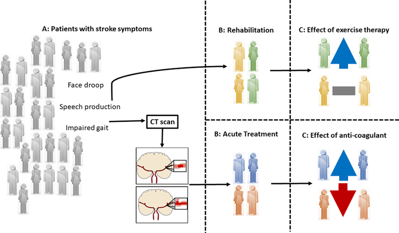
(A) Unlabeled cases (grey) first present with behavioral symptoms like face droop, impaired speech production, or impaired gait. Cases then undergo a CT scan to determine the cause of the stroke. (B) Four cases are labeled based on clinician identified outcomes such as the use of the anti-coagulant, warfarin. Patient are ‘sub-grouped’ into ischemic (blue) or hemorrhagic (red) stroke groups as determined from CT scans. (C) Effect of warfarin treatment on outcome. The effect of anti-coagulants during acute treatment, where anti-coagulants may harm cases with hemorrhagic stroke but benefit cases with ischemic stroke. In this instance, being able to sub-group individuals outside of signs and symptoms is critical for treatment. (D) The same exact cases as in (B); however, cases are now grouped by impaired gait (green) or speech (yellow) as determined from stroke symptoms. (E) The effect of exercise therapy during rehabilitation, which benefits impaired gait but not impaired speech, is also dependent on the distinct sub-grouping (D). Populations, such as stroke populations can be sub-divided into subgroups in many different ways. Which possibility is the most important depends in large part on the question of interest.

Ensemble hybrid approaches may overcome these limitations

Hybrid approaches, such as the functional random forest (FRF) [59], and surrogate variable analysis (SVA) [89] may overcome these limitations by combining the advantages of supervised and unsupervised approaches. The FRF combines a supervised random forest (RF)[90] with an unsupervised community detection algorithm, Infomap[91], to characterize heterogeneity tied to one’s question of interest. SVA combines an unsupervised principal component analysis (PCA) with a supervised learning approach to characterize heterogeneity untied to one’s question of interest. These approaches will be discussed in more detail below.

FRF characterizes biologically relevant heterogeneity and identifies subtypes

The FRF combines machine learning, in this case the RF [90], and graph theoretic analyses, here community detection [92], to characterize relevant heterogeneity and subtypes within populations [59]. The FRF characterizes unknown heterogeneity with respect to a question, combining supervised and unsupervised approaches. The FRF identifies subtypes that are tied to a clinical or cognitive outcome (Figure 4). First, data (called features; Figure 4: red box) are fit to an outcome via a RF model (Figure 4: green box), using cross-validation to assess model performance. A RF model comprises a collection of decision trees (Figure 4: red box). A decision tree is a model that splits cases (nodes) via paths comprising a series of binary rules (paired branches). Cases flow left or right depending on the rule, and multiple paths may lead to the same outcome. The input features can include unstructured clinical notes, clinical assessment or task measures, and even high-dimensional biological data. For example, a decision tree may be formed to determine whether a child may need educational support in school. One branch might split children by IQ, with those less than 70 requiring support. Another might split children by autism diagnosis, with those diagnosed positively requiring support. Critically, each tree is developed randomly. A random subset of the data is used to generate pseudo-random datasets to train each tree. Within each tree, each rule is determined by selecting the rule with the best split from a randomly chosen subset of features. Such random ensembles will ignore features that are noise (with regard to the outcome), unlike the unsupervised approaches above.

Figure 4. FRF identifies subtypes relevant to the question of interest.

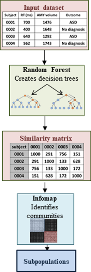
The FRF attempts to identify subtypes tied to a specific outcome or measure. Input datasets (top red panel) are input into a RF algorithm. Input data can comprise measures with any distributions, and can even be categorical. Outcomes may be continuous or categorical variables. Input data are split into testing and training datasets, preferably by 5- or 10-fold cross validation (see Box 1). The RF[90] (green panel) comprises an ensemble of decision trees. Per tree, a subset of the training data is bootstrap resampled and used to construct the decision tree. Per branch, a random subset of measures is selected. The selected measure that best splits the data according to the outcome forms the rule for the given branch. Trees stop growing when data are sufficiently divided into appropriate bins, called “terminal nodes”, reflecting the same or similar outcome measure. Testing data are evaluated for each tree, which votes on the data, and the predicted outcome is calculated by averaging the votes. Individuals may take different paths (red lines) that predict the same outcome. By counting these paths, one can form a similarity matrix (lower red panel) for input or independent datasets, and the matrix reflects the total number of times participants traverse the same paths through the forest. This matrix is recast as a graph and input into an Infomap algorithm[92] (light blue panel), which uses a random walker to identify subtypes (bottom panel).

The RF algorithm produces a similarity/proximity matrix (Figure 4: similarity matrix box), which represents the similarity between pairs of individuals, and a score, which represents the probability of the predicted outcome. The proximity matrix from a given RF is then recast as a graph, where nodes reflect participants and edges are weighted by participant-participant proximity. Community Detection, a graph theory approach (Figure 4: light blue box), is used iteratively to identify subgroups (Figure 4: bottom box). The community detection algorithm used currently is Infomap [93]. Infomap uses a random walker that traverses the constructed graph to identify communities, where a subset of individuals (i.e. nodes) contain more edges that connect each other than edges that do not. The technique is robust to many case scenarios[87]. Because Infomap makes few assumptions regarding the number of groups or their composition, the user does not need to specify how many groups are present, unlike the supervised approaches above. Together these tools represent the FRF.

The outcome for the FRF reflects the question asked by the analysis. In other words, the proximity matrix used to identify whether subtypes exist is built specifically for the predicted outcome variable. If the model performs well, then identified subtypes are likely to be tied to the outcome. For example, an investigator, using the identical data, might define diagnostic subtypes from several clinical variables and demographic variables. Using the same input features distinct subtypes might be drawn from an outcome related to future academic performance, which would weight these features differently. Critically, the FRF makes few assumptions regarding data inputs, and can implicitly handle categorical and continuous data in the same model.

The potential usage of such an approach might be applied to our example on stroke noted in figure 3. Let’s say for example a group of investigators were interested in generating a model that could predict who will benefit from Warfarin for secondary prevention of a subsequent stroke. In this hypothetical example the investigators are unaware of the true mechanisms of the behavioral sequela of stroke, but do know that there is variability with regard to demographics, health history, environmental exposures, symptoms, and CT findings (i.e. hyperintensities, null findings, and hypointesities on the scan) at the time of presentation. They also know that not everyone with stroke benefits from anti-coagulation. At their disposal is a large population of stroke patients with all of their models input features (i.e., demographics, symptoms, etc.) and their long-term outcomes (i.e. prevention of a new stroke or not). This scenario is similar to the current state of affairs of clinical research with regard to mental health conditions. If the investigators used current supervised or unsupervised approaches that do not utilize the outcome of interest (i.e. secondary prevention) to parse the variability across all of the features they would likely identify different types of clusters depending on the restraints and bias of a given method. For example, a supervised approach that was set to force the data into two groups might fit the data primarily into males and females because of the precision of this feature in the data set. This subgrouping is valid, but has limited impact on the outcome of interest. Of course, there are nearly an unlimited number of outcomes depending on the actual type of model used and the specified model parameters; however, such supervised approaches limit the chance that the we identify the model specific to our outcome of interest. Unsupervised models, while not requiring such explicit parameters like the number of groups, is also not guaranteed to give an optimal grouping decision that is important for our question or outcome (i.e. prevention or not when on warfarin).

Under these circumstances, methods like the FRF have an advantage. The investigators using the FRF would utilize all of the same features to generate the model; however, the first stage of the modeling would initially identify whether the features input are capable of predicting the outcome of interest, and then determine which features are important for that prediction (i.e., it would filter out the features of ‘no interest’ related to secondary prevention). For our case, demographic and environmental measures are not associated with secondary prevention and the use of warfarin. Therefore, they would have limited contributions to the predictions and thus would not be highly weighted when identifying sub-populations (i.e. the proximity matrix and community detection sub-grouping would be driven by the CT scan because CT measures contribute most to predicting the outcome of interest; see Figure 3b and c). Importantly, simply changing the outcome of interest (e.g. to exercise therapy effectiveness) would cause the model to weight input features differently (Figure 3d and e). In turn, these differences would inform distinct sub-populations based on the new outcome measure.

The FRF has recently been used in a proof of principal study to identify putative ASD and typical subtypes relevant to an ASD diagnosis[59]. Behavioral data derived from tasks reflecting multiple cognitive domains were used to predict ASD diagnosis in ASD and typical samples. The FRF identified three putative ASD and four putative typical subgroups. Both sets of subgroups showed similar variation in cognitive profiles, suggesting that ASD heterogeneity may be nested within typical heterogeneity. Variation in functional brain organization between the ASD subgroups overlapped with differences between ASD and typical samples, suggesting that these subgroups had biological relevance (Figure 5).

Figure 5. Functional connectivity patterns vary by FRF identified subtype.

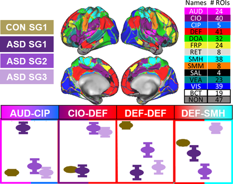
This figure was modified from [59] where the FRF was applied to behavioral data. Sufficient fcMRI data was obtained for three ASD subgroups (ASD SG1, ASD SG2, ASD SG3) and one typical subgroup ( CON SG1 - see legend). A chi-squared analysis was performed, using systems identified by Gordon et al[127] to determine within or between network systems that were differentially atypical amongst these groups (see brain inset). Briefly, the chi-squared analysis tests whether the number of significantly varying connections within or between two communities are greater than what would be observed by chance. Here, the analysis reveals intra- and inter-system effects of subgroup. Seven effects were found that showed varying effects relative to the control group with respect to the ASD subgroups. Four are displayed here. (AUD-CIP) ASD subgroup 1 shows increased connectivity between auditory (AUD) and Cingulo-Parietal (CIP) systems. (CIO-DEF) ASD subgroups 2 and 3 show increased connectivity between Cingulo-opercular (CiO) and default (DEF) systems. (DEF-DEF) All three ASD subgroups show decreased connectivity within the default (DEF) system). (DEF-SMH) ASD subgroup 3 shows elevated connectivity between default (DEF) and somatomotor-hand (SMH) systems, while ASD subgroup 2 shows decreased connectivity. Taken together, these findings highlight differential connectivity patterns that do not reflect simple severity, even though the subgroups were identified from behavioral data.

SVA characterizes biologically irrelevant heterogeneity to uncover subtypes

SVA is a hybrid ensemble approach to heterogeneity that was originally developed to eliminate batch effects in genomics data. The approach is distinct from but analogous to the FRF, which will be described in more detail below. In short, data procured in genomic studies often group or cluster secondary to differences in sample collection methods, sequencing dates, and other reasons not related to true genomic variation [94]. Batch effects are analogous to the heterogeneity problem (see: Box 1), where subtypes that might be identified in samples may be driven by multiple mechanisms; however, in this case the drivers of the subgrouping are irrelevant or unrelated to the specific question being asked. Rather clusters are driven by features that reflect sequence artifacts or dates. The specifics with regard to what is the cause of a given batch effect may be unknown and unable to be modeled by an investigator for removal. SVA solves this problem by first generating a model tied to the question asked in the study. In other words, the model selected depends on the question asked by the user. Residuals from the fitted data are then extracted, which are unrelated to the question or outcome. Therefore, any potential clusters that can be identified in the residuals are highly likely to be batch effects. SVA does not attempt to measure such clusters directly [89]; instead, latent variables representing surrogates of such subgroups are identified in the residuals from the data using PCA, where the combination of these variables is equivalent to the combination of batch effects in aggregate. The residual data is now decomposed into a series of independent linear components, where each component comprises a weighted sum of the data’s features. These components can be controlled for when modeling the data, enabling one to avoid heterogeneity in the samples unrelated to the question of interest. Critically, because the batch effects are not explicitly modeled, SVA can reveal and control for unknown heterogeneity that is not tied to the question of interest [95].

Using the same stroke example above, SVA would first model all of the features as a function of the question of interest – again, secondary prevention of stroke after the use of warfarin. In this case, the original model would obtain a strong correspondence with results related to the CT scan. Residuals from the fitted data would then be extracted, which again, are unrelated to the question or outcome. Latent variables identified in the residuals data using PCA would represent grouping variables in the data that are unrelated to the specific outcome here (e.g. gender, socio-econmic status, behavioral symptoms, etc). These components would then be controlled for when modeling the data, enabling one to avoid heterogeneity in the samples that is unrelated to stroke prevention after Warfarin administration.

Because SVA characterizes heterogeneity unrelated to the question, the approach alone cannot identify meaningful subgroups itself. However, by removing batch effects, SVA combined with subsequent unsupervised approaches better identify subgroups tied to clinical outcomes. For example, in the context of myeloid leukemia[96], SVA enabled subsequent subtyping approaches to correctly identify previously validated subtypes. Removing batch effects via SVA has also helped subsequent unsupervised approaches to uncover overlap between inflammatory markers and common pathways implicated in many diseases[97,98], and identify functional components of tumor causing pathways[99].

There are some limitations for SVA. Unfortunately, because SVA attempts to remove unwanted heterogeneity, the approach cannot identify subtypes without the aid of other approaches[95]. Furthermore, SVA can be potentially misleading if the wrong or incomplete biological variables are modeled with respect to the question. Biological heterogeneity may be removed leading to null or even artefactual results. Despite these limitations, SVA is a powerful tool in characterizing unknown heterogeneity within a dataset because it attempts to characterize heterogeneity with respect to the question of interest.

Heterogeneity problem requires future study on hybrid approaches

Though the heterogeneity problem is not new; the development of ensemble hybrid approaches to overcome the heterogeneity problem are few. The approaches presented above are cross-sectional and exploratory, not longitudinal nor confirmatory (see: Box 4 for how the FRF can be applied to longitudinal data and an approach to confirm subgroups). Furthermore, both of the ensemble techniques shown here have limitations. The SVA may not be suitable for longitudinal data, and may remove biological heterogeneity if the wrong variables are considered. Batch effects tied to a question may contaminate identified subtypes via the FRF, and methods to remove batch effects may actually confound the FRF. In addition, methods to handling missing data are still in development.

Box 4: Longitudinal approaches may help refine psychiatric nosology.

When characterizing heterogeneity in typical or atypical populations, in many cases one should consider the divergence in trajectories (also see Box 2). Future work might incorporate longitudinal methods along with supervised and unsupervised approaches for such purpose. For example, functional data analysis might be used to extend the FRF and characterize heterogeneity from longitudinal trajectories. Functional data analysis (FDA) is a recently introduced method that uses a set of basis functions to identify each individual’s trajectory [123]. In the first stage, piecewise polynomial functions are used to fit the trajectory of each symptom per individual and produce a set of coefficients. In the cases below, 4th order B-splines were used to fit the individual trajectory, and penalized by 2nd order B-splines. Knots are fitted at each of the measured time points. While spline-fitting can handle irregularly collected data, at least 4 timepoints are necessary to estimate trajectories.

To characterize heterogeneity of trajectories from longitudinal data, information from the individual trajectories from FDA can be utilized. Two methods might be used (Figure 6). 1) A similarity matrix can be formed from the trajectories (e.g., subject-subject correlation), and infomap used iteratively to identify subgroups (Figure 6: blue unsupervised pathway), or 2) the parameters of the basis functions for each individual might be input into the random forest and community detection performed on the subsequent proximity matrix (Figure 6: red hybrid pathway).

Concluding Remarks

The heterogeneity problem is an acute challenge for investigators trying to understand physiologic and biologic correlates to typical cognition and mental health. The hybrid approaches highlighted here represent early but critical progress in characterizing heterogeneity in large-scale basic science and clinical studies of complex human behavior.

The work with this regard is still in the early stages, and future development and comparisons across methods are needed amidst various data types used for study of brain and cognition (see: Outstanding Questions). Yet, as we continue to embark on massive endeavors to map the human brain across development and aging, both structurally and functionally[100–103], we feel that characterizing the heterogeneity in typical and atypical populations is likely going to be a major component of these efforts that will have to be improved before we are able to reveal their full potential.

Figure 6. FRF can identify subtypes from longitudinal trajectories.

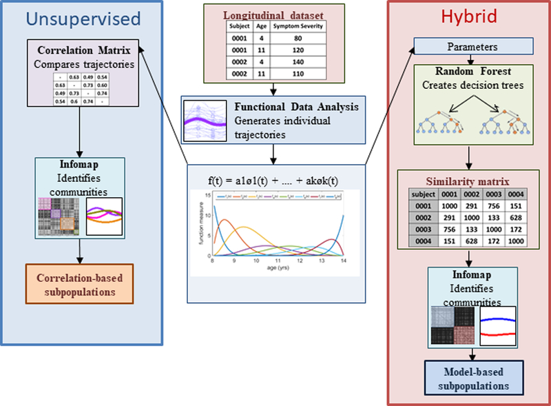
Input dataset (center red panel) comprise at least 4 time points per case. Preferably, the first and last time point occur at the same time across the cases. B-spline basis functions[123] are fit to each case’s time series. (hybrid red panel) Per case, parameters are extracted from the fit functions and entered into the FRF (see: Figure 4). Model-based subtypes identified through this approach can be tied to a question. Subtypes can also be identified through an unsupervised approach (unsupervised blue panel). First, a correlation matrix is produce by calculating the correlation between each case’s predicted trajectory. The correlation matrix is then entered into Infomap, which identifies the correlation based subtypes.

GLOSSARY

ADHD

attention deficit hyperactive disorder. A prevalent developmental disorder characterized by inattentive and/or hyperactive symptoms.

ASD

autism spectrum disorder. A prevalent developmental disorder characterized by altered social communication and restricted interests/repetitive behaviors.

CCM

collaborative care management. A depression study that measured the effects of collaborative care on depression outcomes.

COMED

combining medications to enhance depression outcomes. A depression study that measured the effects of multi-drug treatments on depression outcomes.

CT

Computerized tomography. An imaging approach that uses X-rays to create detailed views of different organs and/or tissues. CT is commonly used to diagnose the cause of strokes.

DCM

dynamic causal modelling. A mixture modelling approach developed to link BOLD activity to neural activity. Modified to identify subtypes within a multi-dimensional space (e.g. RDOC), and help overcome the curse of dimensionality.

DSM

Diagnostic and Statistical Manual for Mental Disorders. A taxonomy for psychiatric/mental health disorders developed by psychiatrists and psychologists within the U.S.

EMC

Early medication change. A depression study that measured the effects of changing medications on depression outcomes.

fcMRI

functional connectivity Magnetic Resonance Imaging. An approach for estimating functional connections between brain regions. The approach involves collecting fMRI data while the participant does not engage in a task. The correlation between spontaneously fluctuating signals derived from two given brain regions indicates the degree of functional connection between them.

fMRI

functional magnetic resonance imaging. Refers to biomarkers derived from functional magnetic resonance imaging studies. Such biomarkers may reflect brain activity in response to a task or stimulus type, or functional connections (see: fcMRI).

FRF

functional random forest. A set of approaches developed into a package to identify subtypes tied to the question of interest. Overcomes limitations of both supervised and unsupervised approaches.

GENDEP

Genome-based therapeutic drugs for depression. A depression study that attempted to identify drug targets for depression based on genomic screening.

HiTOP

Heirarchical Taxonomy of Psychopathology. An unsupervised approach developed by Kotov et al. to identify subtypes organized hierarchically, which may help overcome the curse of dimensionality. Unlike supervised approaches, subtypes are identified based on similarities across large datasets.

ICD

International Classification of Disorders. A taxonomy for pathophysiology. A subset of classifications are for mental health diagnoses.

IQ

intelligence quotient. A standardized metric for measuring both fluid (i.e. how well you learn something) and crystallized (i.e. how much you know) intelligence.

OFC

orbitofrontal cortex. A cortical region associated with many functions, including emotional regulation. Implicated in depression.

PCA

principal component analysis. An approach to decomposing multi-dimensional data into orthogonal components. A key part of the SVA.

PCC

posterior cingulate cortex. A cortical region, which forms part of the Default mode network in the brain. Implicated in depression.

PREDICT

predicting response to depression treatment. A depression study that examined the effects of different treatment regimens on depression outcomes.

RDOC

Research Domain Criteria. A dimensional approach to nosology that characterizes individuals across continuous traits. Developed to help refine psychiatric nosology.

RF

random forest. An ensemble classification approach comprising many decision trees. One of the key parts of the FRF.

sMRI

structural magnetic resonance imaging. Refers to biomarkers derived from anatomical scans, such as T1s and T2s. Such biomarkers often measure shape or size.

SVA

Surrogate variable analysis. An approach and package developed by Leek et al to identify subtypes unrelated to the question of interest (i.e. batch effects). Overcomes limitations of both supervised and unsupervised approaches.

REFERENCES

- 1.Kendler KS (2009) An historical framework for psychiatric nosology. Psychol. Med 39, 1935–1941 [DOI] [PMC free article] [PubMed] [Google Scholar]
- 2.Nigg JT (2006) Temperament and developmental psychopathology. J. Child Psychol. Psychiatry 47, 395–422 [DOI] [PubMed] [Google Scholar]
- 3.Mason D and Hsin H (2018) ‘A more perfect arrangement of plants’: the botanical model in psychiatric nosology, 1676 to the present day. Hist. Psychiatry 29, 131–146 [DOI] [PubMed] [Google Scholar]
- 4.Organization, W.H. and others (1996) Multiaxial classification of child and adolescent psychiatric disorders: the ICD-10 classification of mental and behavioural disorders in children and adolescents, Cambridge Univ Pr. [Google Scholar]
- 5.Robins LN et al. (1981) National Institute of Mental Health Diagnostic Interview Schedule: Its history, characteristics, and validity. Arch Gen Psychiatry 38, 381–389 [DOI] [PubMed] [Google Scholar]
- 6.Robins E and Guze SB (1970) Establishment of diagnostic validity in psychiatric illness: its application to schizophrenia. Am. J. Psychiatry 126, 983–987 [DOI] [PubMed] [Google Scholar]
- 7.Anttila V et al. (2018) Analysis of shared heritability in common disorders of the brain. Science (80-. ) 360, eaap8757. [DOI] [PMC free article] [PubMed] [Google Scholar]
- 8.Wang T et al. (2017) Polygenic risk for five psychiatric disorders and cross-disorder and disorder-specific neural connectivity in two independent populations. NeuroImage Clin 14, 441–449 [DOI] [PMC free article] [PubMed] [Google Scholar]
- 9.Smoller JW et al. (2013) Identification of risk loci with shared effects on five major psychiatric disorders: a genome-wide analysis. Lancet 381, 1371–1379 [DOI] [PMC free article] [PubMed] [Google Scholar]
- 10.Constantino JN and Charman T (2016) Diagnosis of autism spectrum disorder: reconciling the syndrome, its diverse origins, and variation in expression. Lancet. Neurol 15, 279–291 [DOI] [PubMed] [Google Scholar]
- 11.Regier DA et al. (2013) DSM-5 field trials in the United States and Canada, part II: Test-retest reliability of selected categorical diagnoses. Am. J. Psychiatry 170, 59–70 [DOI] [PubMed] [Google Scholar]
- 12.Fried EI (2015) Problematic assumptions have slowed down depression research: Why symptoms, not syndromes are the way forward. Front. Psychol 6, 1–11 [DOI] [PMC free article] [PubMed] [Google Scholar]
- 13.Matthews M et al. (2014) Attention Deficit Hyperactivity Disorder. Curr Top. Behav Neurosci 16, 235–266 [DOI] [PMC free article] [PubMed] [Google Scholar]
- 14.Arbabshirani MR et al. (2017) Single subject prediction of brain disorders in neuroimaging: Promises and pitfalls. Neuroimage 145, 137–165 [DOI] [PMC free article] [PubMed] [Google Scholar]
- 15.Uddin LQ et al. (2017) Progress and roadblocks in the search for brain-based biomarkers of autism and attention-deficit/hyperactivity disorder. Transl. Psychiatry 7, e1218. [DOI] [PMC free article] [PubMed] [Google Scholar]
- 16.Di Martino A et al. (2014) Unraveling the Miswired Connectome: A Developmental Perspective. Neuron 83, 1335–1353 [DOI] [PMC free article] [PubMed] [Google Scholar]
- 17.Cheng W et al. (2018) Increased functional connectivity of the posterior cingulate cortex with the lateral orbitofrontal cortex in depression. Transl. Psychiatry 8, 90. [DOI] [PMC free article] [PubMed] [Google Scholar]
- 18.Fu Z et al. (2018) Transient increased thalamic-sensory connectivity and decreased whole-brain dynamism in autism. Neuroimage 10.1016/j.neuroimage.2018.06.003 [DOI] [PMC free article] [PubMed]
- 19.Marcos-Vidal L et al. (2018) Local functional connectivity suggests functional immaturity in children with attention-deficit/hyperactivity disorder. Hum. Brain Mapp 39, 2442–2454 [DOI] [PMC free article] [PubMed] [Google Scholar]
- 20.de Lacy N et al. (2018) Novel in silico multivariate mapping of intrinsic and anticorrelated connectivity to neurocognitive functional maps supports the maturational hypothesis of ADHD. Hum. Brain Mapp 39, 3449–3467 [DOI] [PMC free article] [PubMed] [Google Scholar]
- 21.Xu Y et al. (2015) Multiple epigenetic factors predict the attention deficit/hyperactivity disorder among the Chinese Han children. J. Psychiatr. Res 64, 40–50 [DOI] [PubMed] [Google Scholar]
- 22.Guo W et al. (2017) Polygenic risk score and heritability estimates reveals a genetic relationship between ASD and OCD. Eur. Neuropsychopharmacol 27, 657–666 [DOI] [PubMed] [Google Scholar]
- 23.Ahn K et al. (2016) Common polygenic variation and risk for childhood-onset schizophrenia. Mol. Psychiatry 21, 94–96 [DOI] [PubMed] [Google Scholar]
- 24.Mistry S et al. (2018) The use of polygenic risk scores to identify phenotypes associated with genetic risk of bipolar disorder and depression: A systematic review. J. Affect. Disord 234, 148–155 [DOI] [PubMed] [Google Scholar]
- 25.Demontis D et al. (2018) Discovery of the first genome-wide significant risk loci for attention deficit/hyperactivity disorder. Nat. Genet 10.1038/s41588-018-0269-7 [DOI] [PMC free article] [PubMed]
- 26.Fair DA et al. (2012) Distinct neuropsychological subgroups in typically developing youth inform heterogeneity in children with ADHD. Proc. Natl. Acad. Sci. U. S. A 109, 6769–74 [DOI] [PMC free article] [PubMed] [Google Scholar]
- 27.Grzadzinski R et al. (2013) DSM-5 and autism spectrum disorders (ASDs): an opportunity for identifying ASD subtypes. Mol. Autism 4, 12. [DOI] [PMC free article] [PubMed] [Google Scholar]
- 28.Cicchetti D (1984) The emergence of developmental psychopathology. Child Dev 55, 1–7 [PubMed] [Google Scholar]
- 29.Xia CH et al. (2018) Linked dimensions of psychopathology and connectivity in functional brain networks. Nat. Commun 9, 3003. [DOI] [PMC free article] [PubMed] [Google Scholar]
- 30.Gaugler T et al. (2014) Most genetic risk for autism resides with common variation. Nat. Genet 46, 881–5 [DOI] [PMC free article] [PubMed] [Google Scholar]
- 31.Saeliw T et al. (2018) Integrated genome-wide Alu methylation and transcriptome profiling analyses reveal novel epigenetic regulatory networks associated with autism spectrum disorder. Mol. Autism 9, 27. [DOI] [PMC free article] [PubMed] [Google Scholar]
- 32.Turner TN et al. (2017) Genomic Patterns of De Novo Mutation in Simplex Autism. Cell 171, 710–722.e12 [DOI] [PMC free article] [PubMed] [Google Scholar]
- 33.Sabuncu MR and Konukoglu E (2014) Clinical Prediction from Structural Brain MRI Scans : A Large-Scale Empirical Study. Neuroinformatics 10.1007/s12021-014-9238-1 [DOI] [PMC free article] [PubMed]
- 34.Katuwal GJ et al. (2016) Divide and Conquer : Sub-Grouping of ASD Improves ASD Detection Based on Brain Morphometry. PLoS One 11, 1–24 [DOI] [PMC free article] [PubMed] [Google Scholar]
- 35.Katuwal GJ et al. (2015) , The Predictive Power of Structural MRI in Autism Diagnosis. , in Annual International Conference of the IEEE Engineering in Medicine and Biology Society, pp. 4270–4273 [DOI] [PubMed] [Google Scholar]
- 36.Chen CP et al. (2015) Diagnostic classification of intrinsic functional connectivity highlights somatosensory, default mode, and visual regions in autism. NeuroImage. Clin 8, 238–45 [DOI] [PMC free article] [PubMed] [Google Scholar]
- 37.Sen B et al. (2018) A general prediction model for the detection of ADHD and Autism using structural and functional MRI. PLoS One 13, e0194856. [DOI] [PMC free article] [PubMed] [Google Scholar]
- 38.Dunlop BW et al. (2017) Functional Connectivity of the Subcallosal Cingulate Cortex And Differential Outcomes to Treatment With Cognitive-Behavioral Therapy or Antidepressant Medication for Major Depressive Disorder. Am. J. Psychiatry 174, 533–545 [DOI] [PMC free article] [PubMed] [Google Scholar]
- 39.Angstman KB et al. (2017) Prediction of Primary Care Depression Outcomes at Six Months: Validation of DOC-6 ©. J. Am. Board Fam. Med 30, 281–287 [DOI] [PubMed] [Google Scholar]
- 40.Wagner S et al. (2017) A combined marker of early non-improvement and the occurrence of melancholic features improve the treatment prediction in patients with Major Depressive Disorders. J. Affect. Disord 221, 184–191 [DOI] [PubMed] [Google Scholar]
- 41.Iniesta R et al. (2016) Combining clinical variables to optimize prediction of antidepressant treatment outcomes. J. Psychiatr. Res 78, 94–102 [DOI] [PubMed] [Google Scholar]
- 42.Chekroud AM et al. (2016) Cross-trial prediction of treatment outcome in depression: a machine learning approach. The lancet. Psychiatry 3, 243–50 [DOI] [PubMed] [Google Scholar]
- 43.Riglin L et al. (2016) Association of Genetic Risk Variants With Attention-Deficit/Hyperactivity Disorder Trajectories in the General Population. JAMA Psychiatry 73, 1285. [DOI] [PMC free article] [PubMed] [Google Scholar]
- 44.Karalunas SL et al. (2014) Subtyping Attention-Deficit/Hyperactivity Disorder Using Temperament Dimensions : Toward Biologically Based Nosologic Criteria. JAMA psychiatry 71, 1015–24 [DOI] [PMC free article] [PubMed] [Google Scholar] [Retracted]
- 45.Fair DA et al. (2013) Distinct neural signatures detected for ADHD subtypes after controlling for micro-movements in resting state functional connectivity MRI data. Front. Syst. Neurosci 6, [DOI] [PMC free article] [PubMed] [Google Scholar]
- 46.Roberts BA et al. (2017) Are there executive dysfunction subtypes within ADHD? J. Atten. Disord 21, 284–293 [DOI] [PMC free article] [PubMed] [Google Scholar]
- 47.Drysdale AT et al. (2017) Resting-state connectivity biomarkers define neurophysiological subtypes of depression. Nat. Med 23, 28–38 [DOI] [PMC free article] [PubMed] [Google Scholar]
- 48.Dinga R et al. (2018) Evaluating the evidence for biotypes of depression: attempted replication of Drysdale et.al. 2017. bioRxiv 10.1101/416321 [DOI]
- 49.Holmes AJ and Patrick LM (2018) The Myth of Optimality in Clinical Neuroscience. Trends Cogn. Sci 22, 241–257 [DOI] [PMC free article] [PubMed] [Google Scholar]
- 50.Yokota S et al. (2015) Individual differences in cognitive performance and brain structure in typically developing children. Dev. Cogn. Neurosci 14, 1–7 [DOI] [PMC free article] [PubMed] [Google Scholar]
- 51.Becht AI et al. (2016) The quest for identity in adolescence: Heterogeneity in daily identity formation and psychosocial adjustment across 5 years. Dev. Psychol 52, 2010–2021 [DOI] [PubMed] [Google Scholar]
- 52.Stapinski LA et al. (2016) Drinking to Cope: a Latent Class Analysis of Coping Motives for Alcohol Use in a Large Cohort of Adolescents. Prev. Sci 17, 584–594 [DOI] [PubMed] [Google Scholar]
- 53.1000 Genomes Project Consortium et al. (2015) A global reference for human genetic variation. Nature 526, 68–74 [DOI] [PMC free article] [PubMed] [Google Scholar]
- 54.Manrique PD and Johnson NF (2018) Individual heterogeneity generating explosive system network dynamics. Phys. Rev. E 97, 32311. [DOI] [PubMed] [Google Scholar]
- 55.Locke J et al. (2016) Examining playground engagement between elementary school children with and without autism spectrum disorder. Autism 20, 653–662 [DOI] [PMC free article] [PubMed] [Google Scholar]
- 56.Locke J et al. (2018) Understanding Friendship Sex Heterophily and Relational Characteristics to Optimize the Selection of Peer Models for Children with Autism Spectrum Disorder. J. Autism Dev. Disord 10.1007/s10803-018-3662-2 [DOI] [PMC free article] [PubMed]
- 57.Morrison AB et al. (2016) Variation in strategy use across measures of verbal working memory. Mem. Cognit 44, 922–936 [DOI] [PMC free article] [PubMed] [Google Scholar]
- 58.Fair DA et al. (2012) Distinct neuropsychological subgroups in typically developing youth inform heterogeneity in children with ADHD. Proc. Natl. Acad. Sci 109, 6769–6774 [DOI] [PMC free article] [PubMed] [Google Scholar]
- 59.Feczko E et al. (2017) Subtyping cognitive profiles in Autism Spectrum Disorder using a random forest algorithm. Neuroimage 10.1016/j.neuroimage.2017.12.044 [DOI] [PMC free article] [PubMed]
- 60.Insel T et al. (2010) Research Domain Criteria ( RDoC ): Toward a new classification framework for research on mental disorders. Am J Psychiatry 167, 748–751 [DOI] [PubMed] [Google Scholar]
- 61.Cuthbert BN and Insel TR (2013) Toward the future of psychiatric diagnosis: the seven pillars of RDoC. BMC Med 11, 126. [DOI] [PMC free article] [PubMed] [Google Scholar]
- 62.Katahira K and Yamashita Y (2017) A Theoretical Framework for Evaluating Psychiatric Research Strategies. Comput. Psychiatry 2, 11–27 [DOI] [PMC free article] [PubMed] [Google Scholar]
- 63.Insel TR The nimh research domain criteria (rdoc) project: Precision medicine for psychiatry. , American Journal of Psychiatry, 171 (2014) , 395–397 [DOI] [PubMed] [Google Scholar]
- 64.Kotov R et al. (2017) The Hierarchical Taxonomy of Psychopathology (HiTOP): A dimensional alternative to traditional nosologies. J. Abnorm. Psychol 126, 454–477 [DOI] [PubMed] [Google Scholar]
- 65.Eysenck SBG et al. (1960) Dimensions of personality, psychiatric syndromes, and mathematical models. J. Ment. Sci 106, 581–589 [DOI] [PubMed] [Google Scholar]
- 66.Achenbach TM (1966) The classification of children’s psychiatric symptoms: a factor-analytic study. Psychol. Monogr. Gen. Appl 80, 1. [DOI] [PubMed] [Google Scholar]
- 67.McConaughy SH et al. (1988) Multiaxial empirically based assessment: Parent, teacher, observational, cognitive, and personality correlates of child behavior profile types for 6-to 11-year-old boys. J. Abnorm. Child Psychol 16, 485–509 [DOI] [PubMed] [Google Scholar]
- 68.Marquand AF et al. (2016) Understanding Heterogeneity in Clinical Cohorts Using Normative Models: Beyond Case-Control Studies. Biol. Psychiatry 80, 552–561 [DOI] [PMC free article] [PubMed] [Google Scholar]
- 69.Hughes G (1968) On the mean accuracy of statistical pattern recognizers. IEEE Trans. Inf. Theory 14, 55–63 [Google Scholar]
- 70.Insel TR (2014) The nimh research domain criteria (rdoc) project: Precision medicine for psychiatry. Am. J. Psychiatry 171, 395–397 [DOI] [PubMed] [Google Scholar]
- 71.Achenbach TM and Rescorla LA (2003) Manual for ASEBA adult forms & profiles, University of Vermont, Research Center for Children, Youth, & Families. [Google Scholar]
- 72.Zimek A et al. (2012) A survey on unsupervised outlier detection in high-dimensional numerical data. Stat. Anal. Data Min 5, 363–387 [Google Scholar]
- 73.Pruett JR and Povinelli DJ Commentary – Autism Spectrum Disorder: Spectrum or Cluster? , Autism Research, 9 December-(2016) , 1237–1240 [DOI] [PMC free article] [PubMed] [Google Scholar]
- 74.Friston KJ et al. (2017) Computational Nosology and Precision Psychiatry. Comput. psychiatry (Cambridge, Mass.) 1, 2–23 [DOI] [PMC free article] [PubMed] [Google Scholar]
- 75.Karalunas SL et al. (2017) Heterogeneity in development of aspects of working memory predicts longitudinal attention deficit hyperactivity disorder symptom change. J. Abnorm. Psychol 126, 774–792 [DOI] [PMC free article] [PubMed] [Google Scholar]
- 76.Karalunas SL et al. (2018) Overlapping and Distinct Cognitive Impairments in Attention-Deficit/Hyperactivity and Autism Spectrum Disorder without Intellectual Disability. J. Abnorm. Child Psychol 10.1007/s10802-017-0394-2 [DOI] [PMC free article] [PubMed]
- 77.Wiggins LD et al. (2017) Homogeneous Subgroups of Young Children with Autism Improve Phenotypic Characterization in the Study to Explore Early Development. J. Autism Dev. Disord 47, 3634–3645 [DOI] [PMC free article] [PubMed] [Google Scholar]
- 78.Huang C et al. (2015) Clustering High-Dimensional Landmark-Based Two-Dimensional Shape Data. J. Am. Stat. Assoc 110, 946–961 [DOI] [PMC free article] [PubMed] [Google Scholar]
- 79.Everitt B and Hand DJ (1981) Finite mixture distributions, Chapman and Hall
- 80.Fair DA et al. (2012) Distinct neuropsychological subgroups in typically developing youth inform heterogeneity in children with ADHD. Proc. Natl. Acad. Sci. USA 109, 6769–6774 [DOI] [PMC free article] [PubMed] [Google Scholar]
- 81.Karalunas SL et al. (2014) Subtyping attention-deficit/hyperactivity disorder using temperament dimensions: Toward biologically based nosologic criteria. JAMA Psychiatry 71, 1015–1024 [DOI] [PMC free article] [PubMed] [Google Scholar] [Retracted]
- 82.Costa Dias TG et al. (2015) Characterizing heterogeneity in children with and without ADHD based on reward system connectivity. Dev. Cogn. Neurosci 11, 155–174 [DOI] [PMC free article] [PubMed] [Google Scholar]
- 83.Gates KM et al. (2014) Organizing Heterogeneous Samples Using Community Detection of GIMME-Derived Resting State Functional Networks. PLoS One 9, e91322. [DOI] [PMC free article] [PubMed] [Google Scholar]
- 84.Lane ST et al. (2018) Uncovering general, shared, and unique temporal patterns in ambulatory assessment data. Psychol. Methods 10.1037/met0000192 [DOI] [PMC free article] [PubMed]
- 85.Wright AG et al. (2017) Focusing personality assessment on the person: Modeling general, shared, and person specific processes in personality and psychopathology. Retrieved from osf.io/nf5me [DOI] [PMC free article] [PubMed]
- 86.Spencer M et al. (2018) Heritable genotype contrast mining reveals novel gene associations specific to autism subgroups. J. Biomed. Inform 77, 50–61 [DOI] [PMC free article] [PubMed] [Google Scholar]
- 87.Gates KM et al. (2016) A Monte Carlo Evaluation of Weighted Community Detection Algorithms. Front. Neuroinform 10, [DOI] [PMC free article] [PubMed] [Google Scholar]
- 88.Everitt B (1993) Cluster analysis, (3rd edn) Arnold E ;Halsted Press. [Google Scholar]
- 89.Leek JT et al. (2012) The sva package for removing batch effects and other unwanted variation in high-throughput experiments. Bioinformatics 28, 882–883 [DOI] [PMC free article] [PubMed] [Google Scholar]
- 90.Breiman LEO (2001) Random Forests. Mach. Learn 45, 5–32 [Google Scholar]
- 91.Rovall M and Bergstrom C. (2008) , Maps of Random Walks on Complex Network Reveal Community Structure. , in Proceedings of the National Academy of Sciences, pp. 105(4), 1118–1123. [DOI] [PMC free article] [PubMed] [Google Scholar]
- 92.Rosvall M and Bergstrom CT (2008) Maps of random walks on complex networks reveal community structure. Proc. Natl. Acad. Sci. U. S. A 105, 1118–1123 %U http://www.ncbi.nlm.nih.gov.beckerpro [DOI] [PMC free article] [PubMed] [Google Scholar]
- 93.Rosvall M and Bergstrom CT (2007) An information-theoretic framework for resolving community structure in complex networks. Proc. Natl. Acad. Sci. U. S. A 104, 7327–7331 %U http://www.ncbi.nlm.nih.gov.beckerpro [DOI] [PMC free article] [PubMed] [Google Scholar]
- 94.Leek JT and Storey JD (2007) Capturing heterogeneity in gene expression studies by surrogate variable analysis. PLoS Genet 3, 1724–1735 [DOI] [PMC free article] [PubMed] [Google Scholar]
- 95.Jaffe AE et al. (2015) Practical impacts of genomic data “cleaning” on biological discovery using surrogate variable analysis. BMC Bioinformatics 16, 372. [DOI] [PMC free article] [PubMed] [Google Scholar]
- 96.Obulkasim A et al. (2015) Subtype prediction in pediatric acute myeloid leukemia: Classification using differential network rank conservation revisited. BMC Bioinformatics 16, 1–11 [DOI] [PMC free article] [PubMed] [Google Scholar]
- 97.Ligthart S et al. (2016) DNA methylation signatures of chronic low-grade inflammation are associated with complex diseases. Genome Biol 17, 1–15 [DOI] [PMC free article] [PubMed] [Google Scholar]
- 98.Fertig EJ et al. (2016) CoGAPS matrix factorization algorithm identifies transcriptional changes in AP-2alpha target genes in feedback from therapeutic inhibition of the EGFR network. Oncotarget 7, [DOI] [PMC free article] [PubMed] [Google Scholar]
- 99.Liu F et al. (2016) Identification of key target genes and pathways in laryngeal carcinoma. Oncol. Lett 12, 1279–1286 [DOI] [PMC free article] [PubMed] [Google Scholar]
- 100.Volkow ND et al. (2017) The conception of the ABCD study: From substance use to a broad NIH collaboration. Dev. Cogn. Neurosci 10.1016/j.dcn.2017.10.002 [DOI] [PMC free article] [PubMed]
- 101.Howell BR et al. (2018) The UNC/UMN Baby Connectome Project (BCP): An overview of the study design and protocol development. Neuroimage 10.1016/j.neuroimage.2018.03.049 [DOI] [PMC free article] [PubMed]
- 102.Schmidt CW Growing a New Study: Environmental Influences on Child Health Outcomes. , Environmental health perspectives, 123 October-(2015) , A260–3 [DOI] [PMC free article] [PubMed] [Google Scholar]
- 103.Cao M et al. (2014) Topological organization of the human brain functional connectome across the lifespan. Dev. Cogn. Neurosci 7, 76–93 [DOI] [PMC free article] [PubMed] [Google Scholar]
- 104.Boyd R (1991) Realism, anti-foundationalism and the enthusiasm for natural kinds. Philos. Stud 61, 127–148 [Google Scholar]
- 105.Zachar P and Kendler KS (2017) The philosophy of nosology. Annu. Rev. Clin. Psychol 13, 49–71 [DOI] [PubMed] [Google Scholar]
- 106.Cicchetti D and Rogosch FA (1996) Equifinality and multifinality in developmental psychopathology. Dev. Psychopathol 8, 597–600 [Google Scholar]
- 107.Gray JA (1980) Ivan Pavlov, Viking Press; New York. [Google Scholar]
- 108.Nigg JT and Barkley RA Attention deficit hyperactivity disorder. In Developmental Psychopathology (Mash E and Barkley RA, eds), Guilford Press [Google Scholar]
- 109.Poland J and Tekin S (2017) Extraordinary science and psychiatry: Responses to the crisis in mental health research, MIT Press. [Google Scholar]
- 110.Kendler KS and Parnas J (2015) Philosophical issues in psychiatry: Explanation, phenomenology, and nosology, JHU Press. [Google Scholar]
- 111.Cuthbert BN and Insel TR (2013) Toward the future of psychiatric diagnosis: the seven pillars of RDoC. BMC Med 11, 126. [DOI] [PMC free article] [PubMed] [Google Scholar]
- 112.Redish AD and Gordon JA (2016) Computational Psychiatry. New Perspect. Ment. Illness, MIT Press [Google Scholar]
- 113.Dosenbach NUF et al. (2010) Prediction of individual brain maturity using fMRI. Science (80-. ) 329, 1358–1361 [DOI] [PMC free article] [PubMed] [Google Scholar]
- 114.Varoquaux G (2017) Cross-validation failure: small sample sizes lead to large error bars. ArXiv e-prints [DOI] [PubMed]
- 115.Breiman L and Spector P (1992) Submodel Selection and Evaluation in Regression. The X-Random Case. Int. Stat. Rev. / Rev. Int. Stat 60, 291–319 [Google Scholar]
- 116.Kohavi R (1995) , A study of cross-validation and bootstrap for accuracy estimation and model selection. , in International Joint Conference on Artificial Intelligence (IJCAI), pp. 1137–1145 [Google Scholar]
- 117.Saeys Y et al. (2007) A review of feature selection techniques in bioinformatics. Bioinformatics 23, 2507–2517 [DOI] [PubMed] [Google Scholar]
- 118.Ransohoff DF (2005) Lessons from Controversy: Ovarian Cancer Screening and Serum Proteomics. JNCI J. Natl. Cancer Inst 97, 315–319 [DOI] [PubMed] [Google Scholar]
- 119.Jamal W et al. (2014) Classification of autism spectrum disorder using supervised learning of brain connectivity measures extracted from synchrostates. J. Neural Eng 11, 046019. [DOI] [PubMed] [Google Scholar]
- 120.Hazlett HC et al. (2017) Early brain development in infants at high risk for autism spectrum disorder. Nature 542, 348. [DOI] [PMC free article] [PubMed] [Google Scholar]
- 121.Crippa A et al. (2015) Use of Machine Learning to Identify Children with Autism and Their Motor Abnormalities. J. Autism Dev. Disord 45, 2146–2156 [DOI] [PubMed] [Google Scholar]
- 122.Abraham A et al. (2016) Deriving reproducible biomarkers from multi-site resting-state data: An Autism-based example. Neuroimage 10.1016/j.neuroimage.2016.10.045 [DOI] [PubMed]
- 123.Ramsay T (2002) Spline smoothing over difficult regions. J. R. Stat. Soc. B 64, 307–319 [Google Scholar]
- 124.Hadi AS (1992) Identifying multiple outliers in multivariate data. J. R. Stat. Soc. Ser. B
- 125.Wickham H (2016) ggplot2: Elegant Graphics for Data Analysis, Springer-Verlag; New York. [Google Scholar]
- 126.code by Richard A Becker OS et al. maps: Draw Geographical Maps. (2018)
- 127.Gordon EM et al. (2014) Generation and Evaluation of a Cortical Area Parcellation from Resting-State Correlations. Cereb. Cortex 26, 288–303 [DOI] [PMC free article] [PubMed] [Google Scholar]
Associated Data
This section collects any data citations, data availability statements, or supplementary materials included in this article.