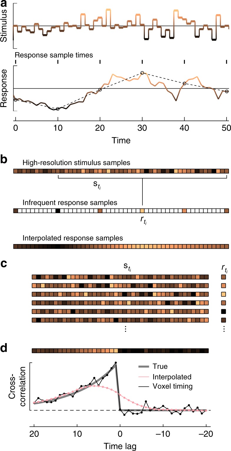
Fig. 2.

Procedure for computing temporal super-resolution cross-correlations. a Stimulus and response used in the numerical simulation. Stimulus values at each time were drawn from a Gaussian distribution. The response was computed as the convolution of the stimulus with an exponential filter with a timescale of 10 timesteps. Color and y-position each indicate the value of the functions. Responses were measured at the black circles; the dashed line represents a linearly interpolated response between measurements. b A vector representation of the stimulus may be constructed so that each element represents the value of the stimulus during that timestep (colors correspond to the value of the signals, as in a). A vector of the sampled response may also be constructed, leaving blank those elements where no measurements were made. The response was sampled every 10 timesteps. An alternate response vector may be constructed by interpolating the responses to generate response estimates during the frames when no measurements were made. For the sampled responses, if responses were measured at the set of times t_i, then the response $r_{t_i}$ may be paired with a snippet of stimulus from the same region, $s_{t_i}$. c The set of (stimulus, response) pairings may be extracted. A simple analysis computes the cross-correlation between stimulus and response, which is an estimate of the linear filter that generates the response. d One finds the cross-correlation by multiplying the response with the stimulus and averaging over all measured responses. The cross-correlation estimate (represented both as a vector at top and a line plot at bottom) is a reasonable estimate of the true filter. When the response is interpolated, the high-resolution filter is not recovered. The time lag is defined as in the text and as in other figures