Figure 2.

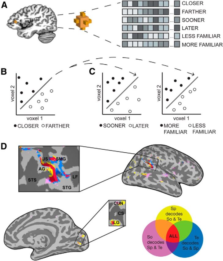
Classification searchlight analysis and results. A–C, Analysis steps. At each voxel, local response patterns corresponding to each condition were extracted (A), and a linear SVM learning algorithm was trained to distinguish trials from one distance domain according to direction of distance change (B), then tested on each of the remaining two distance domains independently (C; for clarity of visualization, dots in B and C represent two-voxel response patterns). This procedure was repeated using all pairwise combinations of distance domains (social, spatial, temporal) as training and testing data, resulting in 6 accuracy maps per participant. D, Results. Accuracy maps from each analysis were tested against chance across participants. Red indicates the conjunction of significant results (p < 0.05, FDR corrected, each test) across all six tests. The largest significant cluster was located in right IPL, encompassing both the AG and SMG, and extending into the posterior temporal lobe, followed by a cluster in medial occipital cortex. Results are projected on the right hemisphere of the AFNI TT_N27 template surface. CUN, Cuneus; CS, calcarine sulcus; JS, intermediate sulcus of Jensen; LF, lateral fissure; LG, lingual gyrus; STS, superior temporal sulcus; Sp, spatial distance; So, social distance; Te, temporal distance.