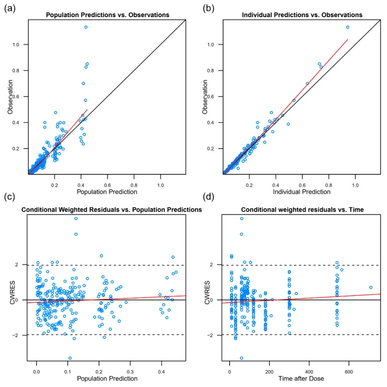
Figure 2.
The goodness-of-fit plots for the population pharmacokinetic model. (a) The observed concentration vs. the population predicted concentration; (b) the observed concentration vs. the individual predicted concentration; (c) the individual weighted residual vs. the individual predicted concentration; (d) the weighted residuals vs. the time. The black lines = the line of identity in (a) and (b) and the line y = 0 in (c,d). The red line = smooth line with locally weighted regression.

