Figure - PMC

Skip to main content

An official website of the United States government

Here's how you know

Here's how you know

Official websites use .gov
A .gov website belongs to an official government organization in the United States.

Secure .gov websites use HTTPS
A lock ( ) or https:// means you've safely connected to the .gov website. Share sensitive information only on official, secure websites.

View full-text article in PMC

. 2019 Nov 1;9:1144. doi: 10.3389/fonc.2019.01144

Search in PMC
Search in PubMed
View in NLM Catalog
Add to search

Copyright © 2019 Heaster, Landman and Skala.

This is an open-access article distributed under the terms of the Creative Commons Attribution License (CC BY). The use, distribution or reproduction in other forums is permitted, provided the original author(s) and the copyright owner(s) are credited and that the original publication in this journal is cited, in accordance with accepted academic practice. No use, distribution or reproduction is permitted which does not comply with these terms.

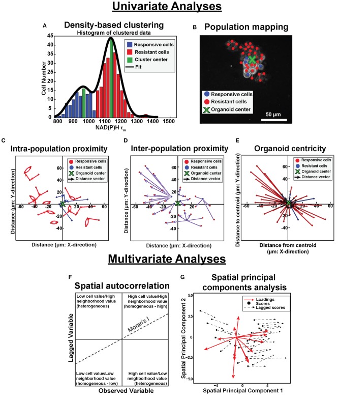
PMC Copyright notice

Population density analysis and spatial statistical analysis quantify spatial heterogeneity of cell metabolism. Single variable analyses using NADH τ_m data is outlined in (A–E). (A) Frequency histograms of single-cell NAD(P)H τ_m values (blue, green, red bars) are fit with kernel density fitting (black line) to represent the data distribution. Density-based clustering analysis of NAD(P)H τ_m identifies sub-populations based on cluster centers (green bins). Cells are assigned to the nearest cluster with higher local density (responsive cluster, blue bins; resistant cluster, red bins). (B) Population spatial maps of NAD(P)H τ_m-defined clusters include markers of responsive cells (blue dots), resistant cells (red dots), and organoid centroid (green x) on top of the original NAD(P)H intensity image (gray). (C) Intra-population proximity is defined as the distance between cells within a population (responsive or resistant), represented by the average length of the blue (responsive) or red (resistant) arrows in the plot. (D) Inter-population proximity is defined as the distances between cells belonging to separate populations (responsive or resistant), represented by the average length of the purple arrows in the plot for the responsive (blue) cells. (E) Organoid centricity is defined as the distance from the organoid center to each cell within a class (responsive or resistant), represented by the average length of the blue (responsive) or red (resistant) arrows in the plot. Multivariate analyses performed across all OMI variables is described in (F,G). (F) Multivariate spatial autocorrelation assesses the similarity of a local cluster by plotting each OMI variable for each cell (observed variable) against the average of its neighboring cells (lagged variable). The slope of the data represents the Moran's I, a global measure of spatial autocorrelation. (G) Multivariate spatial principal components analysis illustrates variation between xenografts and organoids as a function of treatment group and cell population (responsive or resistant). Loadings vectors represent the contribution of each OMI or spatial variable to each spatial principal component (x- and y- axes). Scores for each image are calculated from a linear combination of each variable weighted by their loadings. Lagged scores correspond to the combination of weighted variables for neighbors within an image. Vector lengths represent the average magnitude of difference between cell scores and neighbor (lagged) scores.